Open-Loop Control
As an example of an open-loop controlled system, we look at a mechanical watch. The watch has a problem: it does not know the current time. So during operation it cannot compare setpoint and actual value. Occasionally the wearer looks at a “reference clock”. The wearer uses the time shown there as the setpoint to adjust the time shown on their watch (actual value). That is a brief moment of closed-loop control.
The rotation of the hands of a mechanical watch at the right speed is subject to disturbances. It depends, for example, on temperature, and it changes as the components age. A spring, for example, loses stiffness over the years. Here our predecessors invested a great deal of knowledge of mechanics to reduce this dependence. For example, materials were used on which the disturbances have less effect on the controlled variable. The effect of the disturbances on the controlled variable was reduced so far that the system can be operated in open-loop control.
Electric clocks without an internet connection and without a radio module also solve this problem with open-loop control. They use high-precision quartz crystals that provide a precise clock rate. The influence of disturbances on the controlled variable was reduced even further.
Only with radio-controlled clocks or smartphones did it become possible to provide the clock with the correct time permanently. Now accurate (open-loop) mechanics is no longer needed to show the correct time over a long period with as few external interventions as possible. Now closed-loop control is possible, which always shows the correct time regardless of all disturbances.
The availability of the correct time as a measured value made closed-loop control of the system possible in the first place. As soon as this quantity became available, the change to closed-loop control was made immediately. That is why many modern clocks no longer run open-loop. This is typical of digitalisation: more and more is closed-loop controlled, which is why it is increasingly important to understand control engineering.
Let us look at another example: the fill level h of a tank should match a setpoint. For the example, we assume that the reference variable (setpoint) is hsoll = 1 m. The disturbance in the tank is the outlet through which water is drawn off. In open-loop control, the amount of water flowing out of the tank through the outlet is measured. To keep the fill level at the setpoint, the same amount of water is simply fed back in through the inlet (actuator).
If the reference variable is increased from hsoll = 1 m to, for example, hsoll = 1.1 m, the system must know how to react. For this, a complete calculation model with all the necessary formulas must be stored in the open-loop controller. If the base area A of the tank is known (e.g. A = 1 m2), the necessary change in water volume can be calculated. The following applies:
A water volume of dV = 1 m2 ∙ 0.1 m = 0.1 m3 must be added. The inlet tap is therefore left open until this amount has flowed into the tank. The duration can be determined from the volume flow of the inlet.
The calculations required in an open-loop system can become very complicated. They are carried out in the “open-loop controller” block, which calculates the correct drive signal for the actuator from the measured disturbances. In this example, compensating for the disturbance was relatively simple, while tracking the output quantity when the setpoint changes was relatively complicated. The following block diagram models the task:
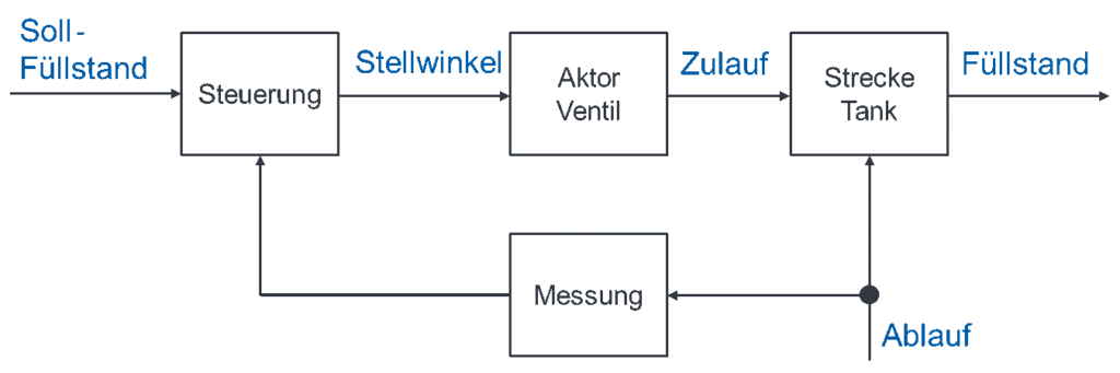
The setpoint “target fill level” specifies what the user wants for the output quantity. It is an input quantity for the block “open-loop controller”. From the setpoint and the measured disturbance “outflow”, this block calculates the correct valve angle for the actuator “valve”. The valve specifies the inflow of water to the tank. The fill level of the tank is determined by inflow and outflow.
For cruise control, open-loop control is much more complicated still. As a reminder: in open-loop control, all disturbances are measured and the input quantity is changed with them so that the output quantity remains equal to the setpoint.
For this example, we assume that a car should drive at 80 km/h. On a straight road it does drive at exactly 80 km/h. The disturbances when setting the speed of a car are mainly gradient and headwind. Let us concentrate on the gradient. Now the car drives up a hill. You measure the gradient of the hill as the disturbance (somehow). The open-loop controller must now know how the accelerator pedal as the input quantity must be adjusted so that the output quantity speed is still 80 km/h.
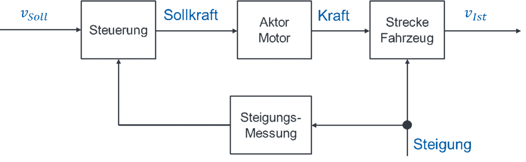
For this, the open-loop controller would have to know the braking effect of the gradient, the engine, the gearbox, the power transmission at the tyres, etc. as formulas. That is impossible in practice. It is also not necessary, because in such cases closed-loop control is used instead of open-loop control. The block diagram of the open-loop control would also have to be extended by the measurement of all further disturbances. We do without that here.
Summary
In open-loop control, all disturbance variables are measured. The measurements are recorded by a control unit. In general, the setpoint is also called the “reference variable”. From the reference variable and all measured disturbances, the open-loop controller calculates the actuator drive signal with which output quantity = reference variable is achieved. In general, open-loop controlled systems are modelled as follows:
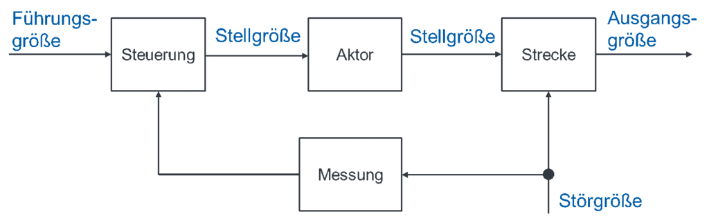
All open-loop controlled systems are modelled in the same way. The same standard blocks are used each time. The blocks are only filled with different terms for each example.