Control Engineering › Controlled Systems

Dynamic Behavior

With P behaviour, the transfer function is a constant. In general, transfer functions can be time-dependent. With a constant input, the output of a system then changes over time t. We recognise this by the fact that the time t appears in the formula for H.

Time dependence is measured and characterised with the step response. For this, a step in the input quantity from 0 to a constant value (e.g. input = 1) is applied at the input of the system. For the gearbox, the rotational speed N₁ is changed in a step from 0 revolutions per minute (unit rpm, “revolutions per minute”) to 1 rpm. Assuming the transfer function of the gearbox had the value H = 10, the output shaft would turn ten times as fast as the input shaft. The output shaft would thus jump from N₂ = 0 rpm to N₂ = 10 rpm.

Proportional systems react at the output directly to changes at the input. There is no time shift or delay. For a step at the time t = 1 s, the step response of this gearbox with (an assumed) H = 10 looks like this:

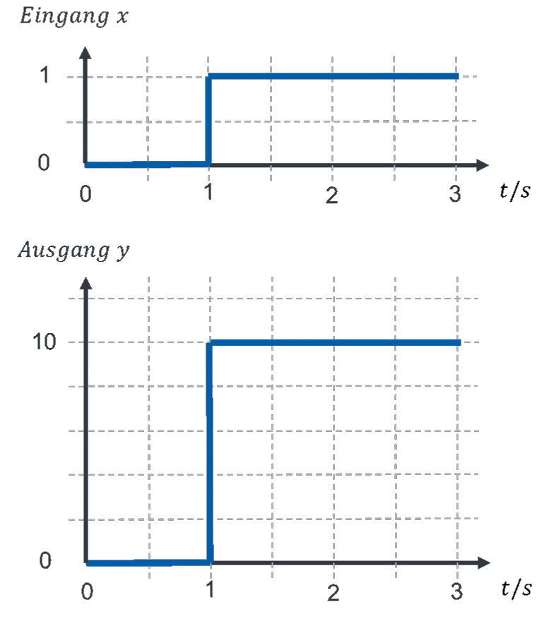
Step at input x at t = 1 s and step response of output y to the value 10 — Eingang = input · Ausgang = output

The point of the step response only becomes clear with other, time-dependent behaviours. I introduce the step response here using a simple example.

Benefit of the step response

With P behaviour, we took one pair of values and used it to determine the characteristic parameter. If the transfer function is time-dependent, this no longer works. That is why we always use the step response to recognise the behaviour of a function block and to determine its characteristic parameters. So far we have only met the parameter k_P for P behaviour. We can determine it from the step response as well.

With the step response, we determine the characteristic parameters without knowing the internal structure, just by measuring the external quantities. That is great, because it means that in future we can control systems without understanding them. This is particularly helpful for complex systems such as a car. As an example, we take a lever whose arm lengths we do not know and cannot (or do not want to) measure.

We deflect the input of the system (the height h₁) abruptly from 0 cm to 1 cm. Then we measure how the output behaves. If it jumps from the deflection 0 to a constant output value without delay, the system behaves proportionally. To characterise the system, we then still need the value k_P. You determine it from the quotient of output value and input value. If, for example, the output value changes by 10 cm, you can calculate the proportional coefficient as follows:

\[ \begin{gathered} H = \frac{\text{output}}{\text{input}} = \frac{h_2}{h_1} = \frac{10\,\mathrm{cm}}{1\,\mathrm{cm}} = 10 \\[6pt] H \text{ constant} \rightarrow \text{P behaviour} \rightarrow k_P = H = 10 \end{gathered} \]

For the step response, we only need the system, a measurement of the input and output quantities and the possibility of exciting it at the input with a step.

You can determine the behaviour of a car and its characteristic parameters by changing its input quantity, the pedal position, in a step from 0 to full throttle. Then you measure the output quantity speed over time. This lets you learn a lot about the behaviour of the car in a control loop without having to understand the engine or the gearbox. I find that brilliant.

Step height

The height of the step at the input is arbitrary. Why do we always step the input from 0 to 1? This has to do with the transfer function.

\[ \begin{gathered} H = \frac{\text{output}}{\text{input}} \\[6pt] \text{with input} = 1 \rightarrow H = \text{output} \end{gathered} \]

If the input equals 1, the output corresponds directly to the transfer function H. We save one calculation step. So if we look at the time behaviour of the output for a step from 0 to 1, we see the time behaviour of the transfer function directly in the output.

If a step from 0 to 1 is not possible, you can step to any other value. If, for example, you step from 0 to 2, you have to divide the output by 2 and then have the transfer function. This follows directly from the formula relating input, output and transfer function.