Electrical Engineering BMT & UFC › Alternating Current

AC Voltage

The alternating voltage at a mains socket u(t) can be described with the sine mathematics from the previous chapter. In the next step, the formula of numbers b(t) is transferred to a voltage u(t) with units. To do this, the equation is multiplied by a voltage.

\[ \begin{gathered} b(t) = \sin\left(\frac{2\pi}{T} \cdot t\right) \text{ with range } b(t) = [-1 \ldots 1] \\[6pt] \text{In general: } u(t) = \hat{u} \cdot \sin\left(\frac{2\pi}{T} \cdot t\right) \text{ with range } [-\hat{u} \ldots \hat{u}] \\[6pt] \text{Example with } \hat{u} = 325\,\mathrm{V}\text{: } u(t) = 325\,\mathrm{V} \cdot \sin\left(\frac{2\pi}{T} \cdot t\right) \text{ with range } [-325\,\mathrm{V} \ldots 325\,\mathrm{V}] \end{gathered} \]

The factor gives the general sine a technical meaning. A voltage curve is given a factor in front of the sine that contains the maximum value of the voltage and the unit volt. The radius of the circle thus no longer has the value 1 but the value 325 V. The peak value (325 V in the example) determines the maximum and minimum value of the voltage. You can calculate intermediate values of the voltage between the extreme values by substituting t into the equation.

Why do I use the odd value of 325 V in the example? Because that is the peak value of the alternating voltage at a German mains socket.

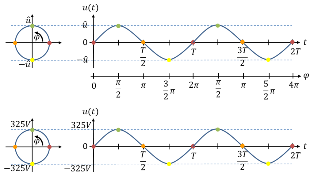
Alternating voltage u(t) with peak value û in general and with û = 325 V

The time curve of the voltage is shown over two periods T in the figure above. An alternating voltage does not stop oscillating after one period; it generally continues to oscillate over a great many periods. The voltage at the mains socket has been oscillating up and down for more than 100 years.

As the next step, we free the time axis from the period T. When you measure time curves of real alternating voltages, the x-axis shows real time values. For this, we need the concept of frequency.

Frequency

The frequency f indicates how often an event occurs per unit of time. Let us take the term “beats per minute” from music. It indicates how many bass beats occur per minute in a song. The faster the song, the more beats occur per minute. This already represents a frequency. 120 beats per minute correspond to 2 beats per second. In engineering, frequency is always related to one second.

In AC engineering, the concept of frequency is used to count how many periods a signal has per second, i.e. how often the signal b(t) goes around the circle per second. Frequency is given in the unit hertz (Hz). This corresponds to the SI unit [Hz] = 1/s. The voltage from a European mains socket has the frequency f = 50 Hz. This means that the voltage passes through 50 complete periods of the sine per second. If 50 periods fit into one second, one period lasts one fiftieth of a second. The period is linked to the frequency. The following applies

\[ \begin{gathered} T = \frac{1}{f},\ [T] = \mathrm{s} \\[6pt] f = \frac{1}{T},\ [f] = \mathrm{Hz} = \frac{1}{\mathrm{s}} \\[6pt] \text{Example mains socket: } f = 50\,\mathrm{Hz} \rightarrow T = \frac{1}{f} = \frac{1}{50\,\mathrm{Hz}} = 20\,\mathrm{ms} \end{gathered} \]

The formula also fits in terms of units, because the period is a time given in seconds. The frequency is given in hertz, i.e. in 1/s. The voltage at the mains socket with f = 50 Hz shows the following time curve over two periods:

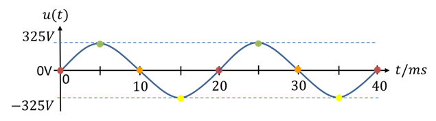
Mains voltage with 325 V peak value and 20 ms period

\[ u(t) = 325\,\mathrm{V} \cdot \sin\left(\frac{2\pi}{T} \cdot t\right) \]

Let us mentally sit on the sine function in the figure above and let the time t pass. Over time, the voltage moves back and forth along the function between the minimum and the maximum voltage value. For every point in time t, there is an associated voltage value u(t), which can either be read off graphically from the figure or calculated mathematically with the formula. This momentary voltage value is called the instantaneous value. The magnitude of the extreme values of the curve is the peak value (also called the amplitude).

A frequency is often illustrated as the pitch of a tone. A loudspeaker consists of a vibrating membrane that moves air. The membrane is moved by an electromagnet or piezo element whose deflection is proportional to the voltage. The sound produced therefore depends on the voltage at the loudspeaker.

The intensity of the sound – i.e. its loudness – changes with the peak value of the voltage. The pitch changes with the frequency of the voltage. More on this under this link (in German).

Angular frequency

The angular frequency ω is less intuitive than the frequency f. It describes the angle covered per second, i.e. the number of complete revolutions of length 2π per second multiplied by 2π. The following applies

\[ \begin{gathered} \omega = 2\pi f \\[4pt] f = \frac{1}{T} \\[4pt] \omega = \frac{2\pi}{T} \end{gathered} \]

Physical quantity	Symbol	Unit name	Unit symbol
Frequency	\(f\)	Hertz	\(\mathrm{Hz} = 1/\mathrm{s}\)
Angular frequency	\(\omega\)	per second	\(1/\mathrm{s}\)

Actually, we do not need another frequency quantity. The frequency f would be sufficient to describe everything in electrical engineering. Nevertheless, the angular frequency ω is used in many places in practice. It makes the formula for describing AC quantities simpler, because the term 2π is omitted:

\[ \begin{gathered} u(t) = \hat{u} \cdot \sin\left(\frac{2\pi}{T} \cdot t\right) \\[6pt] \omega = \frac{2\pi}{T} \\[6pt] u(t) = \hat{u} \cdot \sin(\omega t) \end{gathered} \]

Unfortunately, the unit of the angular frequency is not Hz but [ω] = 1/s. Although this is the same SI unit as for the frequency f, the angular frequency ω must always be given in 1/s and the frequency f in Hz (also in the exam).

Phase angle

So far, we have assumed that the voltage curve also has the angle φ = 0 at the time t = 0 s. In general, this is not the case. There is no real zero point of time. That might be the moment of the Big Bang, but certainly not some time at which a sinusoidal voltage begins. As with electric potentials, we choose the reference point of time freely. For voltages and potentials, we defined ourselves which potential the ground has as the reference point. We can then calculate with this arbitrary definition.

We can choose the zero point or reference point of time freely. The mains voltage passes through 50 periods per second. At which time t we begin the mathematical description is arbitrary. So we can place the zero point of time wherever it suits us best mathematically. We can place it so that all sinusoidal quantities without a shift begin at t = 0 s with φ = 0.

If two sinusoidal curves are present at the same time and are shown in one graph, they can be shifted in time relative to each other. The shift is always the same, regardless of the reference point chosen. It does not matter where we start drawing the curves; they are shifted relative to each other. A time shift by the time t corresponds to a change by an angle φ on the circle. Here is an example of two alternating voltages, each with a peak value of 1 V:

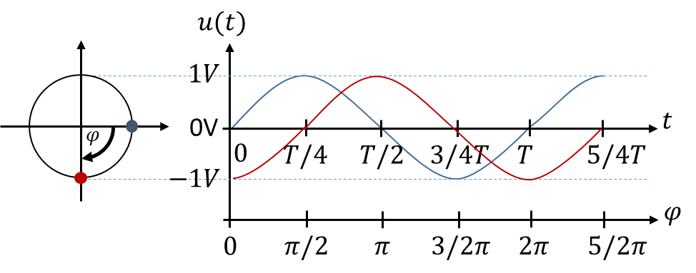
Two sinusoidal voltages with different phase (blue and red)

The red voltage curve is shifted to the “right” by Δφ = −π/2 relative to the blue curve. We also say that the red curve “lags” the blue one in time. The blue curve “leads” the red one. On the time axis on the right, this is a shift by a quarter period towards the future. In the circle representation on the left, this corresponds to a rotation by 90° or π/2 clockwise.

Mathematically, we describe such shifts by adding the angle to the argument of the sine:

\[ \begin{gathered} \text{In general: } u(t) = 1\,\mathrm{V} \cdot \sin(\omega t + \varphi) \\[4pt] \text{Example: } u_{\mathrm{blue}}(t) = 1\,\mathrm{V} \cdot \sin(\omega t + 0) \\[4pt] u_{\mathrm{red}}(t) = 1\,\mathrm{V} \cdot \sin(\omega t - \pi/2) \end{gathered} \]

Why is the shift angle of the red curve negative when the curve is shifted to the right? Intuitively, we would add an angle. Let us substitute a time value whose result we know into the formula. This works best with times if the expression ωt is replaced by 2π/T again. We check whether the formula takes the value U = 1 V expected from the graph at the time t = T/2.

\[ \begin{aligned} u_{\mathrm{red}}\left(t = \frac{T}{2}\right) &= 1\,\mathrm{V} \cdot \sin\left(\frac{2\pi t}{T} - \frac{\pi}{2}\right) = 1\,\mathrm{V} \cdot \sin\left(\frac{2\pi \cdot \frac{T}{2}}{T} - \frac{\pi}{2}\right) \\[6pt] &= 1\,\mathrm{V} \cdot \sin\left(\pi - \frac{\pi}{2}\right) = 1\,\mathrm{V} \cdot \sin\left(\frac{\pi}{2}\right) = 1\,\mathrm{V} \end{aligned} \]

Evidently, the formula reproduces the curve from the graph correctly. If the angle is added (instead of subtracted), the result is wrong. Calculate this as an exercise.

If a curve is shifted to the left relative to the (arbitrarily chosen) zero point of time, a positive angle must be added in the argument of the sine. If the curve is shifted to the right in time, a positive angle is subtracted. Please make sure that we always calculate in “RAD”, never in “DEG” (also in the exam). Please set your calculator accordingly.

The argument of the sine (i.e. the term in its brackets) is always an angle. It has no unit. That is why we cannot simply write a time shift Δt into the argument of the sine. We have to convert it into a phase shift. The following applies:

\[ \varphi = -\frac{\Delta t}{T} \cdot 2\pi \]

The proportion of the shift time in the period, Δt/T, is multiplied by a complete revolution of 2π. This gives us the phase shift for a time shift. Please note the minus sign in the formula.

In practice, two relationships between sine and cosine are also important:

\[ \begin{gathered} u_1(t) = \hat{u}_1 \cos(\omega t) = \hat{u}_1 \sin\left(\omega t + \frac{\pi}{2}\right) \longrightarrow \textbf{cos} \text{ leads } \textbf{sin} \text{ by } \pi/2 \\[6pt] u_2(t) = \hat{u}_2 \sin(\omega t) = \hat{u}_2 \cos\left(\omega t - \frac{\pi}{2}\right) \longrightarrow \textbf{sin} \text{ lags } \textbf{cos} \text{ by } \pi/2 \end{gathered} \]

In this tutorial, we only calculate curves of sinusoidal voltages and currents. Other waveforms are not considered.

As long as we only consider one sinusoidal quantity, specifying a phase angle φ is not helpful. We then always intuitively place the reference point so that φ = 0. This is possible because the voltage at the mains socket has no beginning in time; it is always there and was there before any of us were born. When we measure it or display it graphically, we define a zero point of time for this process.

If we consider more than one sinusoidal quantity and these are shifted in time relative to each other, we need a phase φ to express the shift.

Determining the phase

There is a method for determining the phase shift relative to a zero point of time. With this method, you first determine the period T of a signal. This is the time after which the signal repeats. Then you draw a second angle axis below the time axis. The angle range [0 … 2π] is placed so that it corresponds to the time range [0 .. T].

Then you determine the positive zero crossing of the sine. The sine has two zero crossings. Once it passes through 0 from positive to negative values. That is the wrong one, the negative zero crossing. You are looking for the zero crossing at which the sign of the values changes from negative to positive.

Then you read off the angle at which the sine has its positive zero crossing. This angle with a negative sign equals the phase shift of the function. You have to use a negative sign because you have determined the shift to the right.

The following example illustrates the procedure:

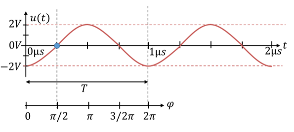
Determining the phase angle from the time curve

\[ \varphi = -\frac{\pi}{2} \]

The angle is always 2π-periodic. An angle of π/2 also corresponds to the angle −3π/2. You can go around the circle anticlockwise by π/2 or clockwise by 3π/2. You end up at the same point. That is why you can always add 2π to the phase shift or subtract 2π from it. It does not change the information contained in the phase shift.

Other AC quantities

Not only the voltage can be an AC quantity. Current and power can also be AC quantities. For the mathematical description, we then use other factors. Examples of sinusoidal alternating current and alternating power are:

\[ \begin{gathered} i(t) = \hat{\imath} \cdot \sin(\omega t + \varphi) \\[4pt] p(t) = \hat{p} \cdot \sin(\omega t + \varphi) \end{gathered} \]

We calculate with these quantities in exactly the same way as with alternating voltages. They are also drawn in the same way.

Example

A sinusoidal voltage curve is given as a formula and shown over time as follows:

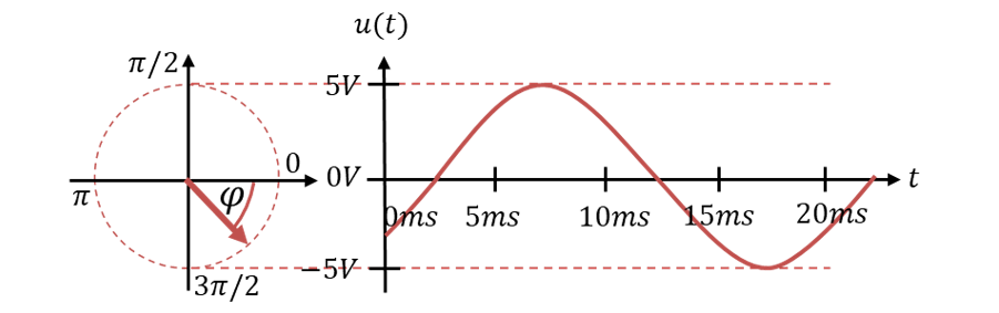
\[ u(t) = 5\,\mathrm{V} \cdot \sin(\omega t + \varphi) \text{ with } T = 20\,\mathrm{ms},\ f = 50\,\mathrm{Hz},\ \omega = 314\,\frac{1}{\mathrm{s}} \text{ and } \varphi = -\frac{\pi}{4} \]

Phasor and time curve of the example voltage

The pointer on the circle in the left part of the picture starts at the position shown. The starting angle indicates the time delay of the signal. The pointer will only reach the zero point of its rotation after 2.5 ms. The peak value of the voltage corresponds to the radius of the circle. The instantaneous value at a time t is determined by projecting the arrow onto the y-axis. Over time t, the pointer moves anticlockwise along the circle. The larger the angular frequency ω, the faster the pointer rotates.

Summary

We have used the following parameters to describe the alternating voltage:

\[ \begin{gathered} u(t) = \hat{u} \cdot \sin(\omega t + \varphi) \\[6pt] \begin{aligned} u(t)&\text{: instantaneous value} \\ \hat{u}&\text{: peak value (amplitude)} \\ \omega&\text{: angular frequency} \\ f&\text{: frequency} \\ t&\text{: time} \\ \varphi&\text{: phase} \end{aligned} \end{gathered} \]

Exercises

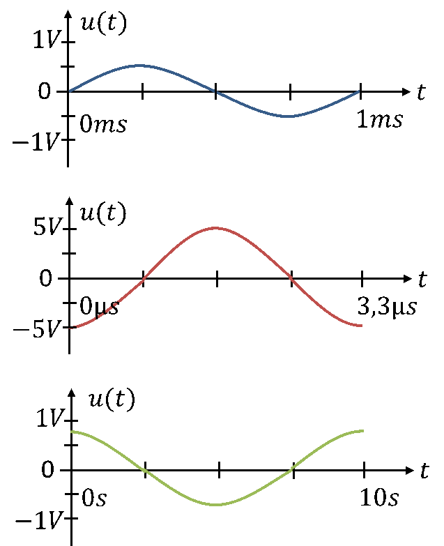
As examples, I give three further voltage curves. Please try to work out the formulas describing them yourself. You will find the solutions further below. Only one period is shown as an excerpt in each case; the curves continue to the left and right exactly as drawn.

Three problems: sinusoidal voltages with different amplitude, period and phase

Solution:

\[ \begin{gathered} u_{\mathrm{blue}}(t) = 0.5\,\mathrm{V} \cdot \sin(\omega t + \varphi) \text{ with } T = 1\,\mathrm{ms},\ f = 1\,\mathrm{kHz},\ \omega = 6.28\,\mathrm{k}\frac{1}{\mathrm{s}} \text{ and } \varphi = 0 \\[6pt] u_{\mathrm{red}}(t) = 5\,\mathrm{V} \cdot \sin(\omega t + \varphi) \text{ with } T = 3.3\,\text{µs},\ f = 300\,\mathrm{kHz},\ \omega = 1.89\,\mathrm{M}\frac{1}{\mathrm{s}} \text{ and } \varphi = -\frac{\pi}{2} \\[6pt] u_{\mathrm{green}}(t) = 0.75\,\mathrm{V} \cdot \sin(\omega t + \varphi) \text{ with } T = 10\,\mathrm{s},\ f = 100\,\mathrm{mHz},\ \omega = 628\,\mathrm{m}\frac{1}{\mathrm{s}} \text{ and } \varphi = \frac{\pi}{2} \end{gathered} \]