Electrical Filters

This chapter is relevant for the exam again. References to the previous chapter may appear. This chapter derives mathematically how filters work.

We can rebuild the water model with electrical components. It then consists of an ideal voltage source (source), a resistor (pipe) and a capacitor (bucket). The voltage source is an AC voltage source. The signal to be filtered is generated by this source. The components are connected in series. We first derive that this series circuit has a filtering effect, i.e. shows frequency-dependent behaviour.

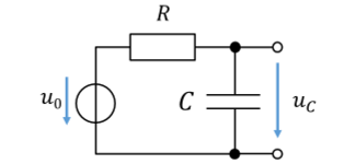
RC low-pass filter of source u_0, resistor R and capacitor C, and filter block from u_0 to u_C

\[ H = \frac{u_C}{u_0} \]

The input quantity of the filter is the source voltage u₀. The output quantity is the voltage across the capacitor u_C. Again we can give a transfer function H. We consider filters only in the frequency domain, never in the time domain. For the output of the filter circuit we need the voltage across the capacitor.

Important: in the chapter on filters, we work both with complex impedances (ETR) and with reactances (BMT and UFC). Students from UFC and BMT did not learn complex impedances in electrical engineering. The texts are split according to the mathematics used. Complex AC calculation (ETR) is in the red box and the simplified calculation with reactances (BMT and UFC) in the blue box. You only need to read the text intended for you.

H with impedances

RC low-pass filter with input voltage u_Ein and output voltage u_Aus — Ein = in (input)

\[ \begin{gathered} \text{Voltage divider: } \underline{u}_{\mathrm{Aus}} = \underline{u}_{\mathrm{Ein}} \cdot \frac{\underline{Z}_C}{\underline{Z}_C + \underline{Z}_R} \\[6pt] \underline{H} = \frac{\underline{u}_{\mathrm{Aus}}}{\underline{u}_{\mathrm{Ein}}} = \frac{\underline{Z}_C}{\underline{Z}_C + \underline{Z}_R} = \frac{\frac{1}{j\omega C}}{R + \frac{1}{j\omega C}} = \frac{1}{1 + j\omega RC} = \frac{1}{1 + j2\pi f \cdot RC} \end{gathered} \]

For the second transformation, I multiplied the numerator and denominator of the fraction by jωC. Since the factor ω appears in the equation, the behaviour of the filter evidently depends on the frequency ω = 2πf.

We are only interested in the magnitude of the transfer function. The phase only indicates a time shift between output and input signal. The magnitude acts on the peak value; it amplifies or attenuates signals. For the magnitude, the real part and imaginary part are added in quadrature:

\[ \begin{gathered} \underline{H} = \frac{\underline{u}_{\mathrm{Aus}}}{\underline{u}_{\mathrm{Ein}}} \\[6pt] \text{Peak values: } |\underline{H}| = \frac{\hat{u}_{\mathrm{Aus}}}{\hat{u}_{\mathrm{Ein}}} \\[6pt] |\underline{H}| = \left|\frac{1}{1 + j\omega RC}\right| = \frac{1}{\sqrt{1^2 + (\omega RC)^2}} = \frac{1}{\sqrt{1 + (\omega RC)^2}} \\[6pt] \hat{u}_{\mathrm{Aus}} = \frac{1}{\sqrt{1 + (\omega RC)^2}} \cdot \hat{u}_{\mathrm{Ein}} \end{gathered} \]

The magnitude of the transfer function indicates how the peak value of the output voltage changes when a sinusoidal input voltage is applied. When the frequency is high, the denominator of the fraction becomes larger and the peak value of the output voltage is smaller. At low frequency, the denominator is small and the output voltage is larger.

Using the magnitude has an advantage: there are no more complex numbers. With the magnitude we can bring the BMT students back on board, who have to manage without complex numbers. ETR students, please skip the next part and rejoin at Dividing into ranges.

H with reactances

We do not need an ideal voltage source at the input, only an input voltage. This makes the definition of the filter more general. The capacitor and resistor form a voltage divider with reactances. Remember: the reactances of resistor and capacitor are added in quadrature. With reactances we can calculate how the peak value of a sinusoidal voltage changes.

\[ \begin{gathered} \text{Voltage divider (magnitudes): } \hat{u}_{\mathrm{Aus}} = \hat{u}_{\mathrm{Ein}} \cdot \frac{X_C}{\sqrt{R^2 + X_C^2}} \\[6pt] H = \frac{\hat{u}_{\mathrm{Aus}}}{\hat{u}_{\mathrm{Ein}}} = \frac{X_C}{\sqrt{R^2 + X_C^2}} = \frac{\frac{1}{\omega C}}{\sqrt{R^2 + \left(\frac{1}{\omega C}\right)^2}} = \frac{1}{\sqrt{1^2 + (\omega RC)^2}} = \frac{1}{\sqrt{1 + (\omega RC)^2}} = \frac{1}{\sqrt{1 + (2\pi f \cdot RC)^2}} \end{gathered} \]

For the second transformation, I multiplied the numerator and denominator of the fraction by ωC. Since the factor ω appears in the equation, the behaviour of the filter evidently depends on the frequency ω = 2πf.

The transfer function acts on the peak value; it amplifies or attenuates signals. To be able to continue compatibly with the ETR students, from now on we use the magnitude of the transfer function. For you it is identical to the transfer function itself; in complex AC calculation we need the magnitude so that everything is mathematically correct. We also no longer use the peak values of the voltages but the voltages in general. Please simply get used to the new notation, which is no longer exactly the same as in electrical engineering:

\[ \begin{gathered} \hat{u}_{\mathrm{Aus}} = H \cdot \hat{u}_{\mathrm{Ein}} \rightarrow u_{\mathrm{Aus}} = |H| \cdot u_{\mathrm{Ein}} \\[6pt] |H| = \frac{u_{\mathrm{Aus}}}{u_{\mathrm{Ein}}} = \frac{1}{\sqrt{1 + (\omega RC)^2}} \\[6pt] \hat{u}_{\mathrm{Aus}} = \frac{1}{\sqrt{1 + (\omega RC)^2}} \cdot \hat{u}_{\mathrm{Ein}} \end{gathered} \]

Dividing into ranges

From here on, we continue together for all degree programmes, regardless of the mathematics chosen. Two ranges are distinguished in the formula:

Range 1: for very low frequencies, 1 ≫ ωRC applies in the denominator of the fraction. If ω on the right-hand side of the equation is small enough, the 1 is much larger. So the term ωRC can be neglected compared with the 1. For very low frequencies we therefore omit it from the formula. The fraction then becomes:

\[ \begin{gathered} |H| = \frac{1}{\sqrt{1 + (\omega RC)^2}} \\[6pt] \text{Range 1: } 1 \gg \omega RC \\[6pt] H(\omega) = \frac{u_{\mathrm{Aus}}(\omega)}{u_{\mathrm{Ein}}(\omega)} = \frac{1}{\sqrt{1 + (\omega RC)^2}} \approx \frac{1}{1} = 1 \\[6pt] u_{\mathrm{Aus}}(\omega) = H(\omega) \cdot u_{\mathrm{Ein}}(\omega) = u_{\mathrm{Ein}}(\omega) \end{gathered} \]

Then u_Aus = u_Ein applies. Signals with very low frequency therefore pass through the filter unchanged.

Range 2: in the other case we consider very high frequencies with 1 ≪ ωRC in the denominator of the fraction. If ω on the right-hand side of the equation is chosen large enough, the 1 is much smaller than this right-hand term. This time we neglect the 1 and omit it. The transfer function can be simplified to

\[ \begin{gathered} \text{Range 2: } 1 \ll \omega RC \\[6pt] H(\omega) = \frac{u_{\mathrm{Aus}}(\omega)}{u_{\mathrm{Ein}}(\omega)} = \frac{1}{\sqrt{1 + (\omega RC)^2}} \approx \frac{1}{\omega RC} \sim \frac{1}{\omega} \\[6pt] u_{\mathrm{Aus}}(\omega) = H(\omega) \cdot u_{\mathrm{Ein}}(\omega) = \frac{1}{\omega RC} \cdot u_{\mathrm{Ein}}(\omega) \\[6pt] \text{Reduction of the peak value by } \frac{1}{\omega RC} \end{gathered} \]

The transfer function decreases with increasing angular frequency ω. So with a constant input voltage, the output voltage decreases with 1/ω. This corresponds to the behaviour f(x) = 1/x from school mathematics. The output signal is rotated in phase by −90° (factor −j). Over time it is shifted to the right relative to the input signal. This matches the reasoning from the water model.

Cut-off frequency

At the point ωRC = 1, the behaviour changes. We call the frequency at which this equation is satisfied the cut-off frequency ω_g. The following applies:

\[ \begin{gathered} \omega RC = 1 \\[6pt] \omega_g = \frac{1}{RC} \end{gathered} \]

We obtain the transfer function at the cut-off frequency by inserting the cut-off angular frequency into the formula of the transfer function:

\[ \begin{gathered} \omega_g = \frac{1}{RC} \\[6pt] H(\omega_g) = \frac{1}{\sqrt{1 + (\omega_g \cdot R \cdot C)^2}} = \frac{1}{\sqrt{1 + \left(\frac{RC}{RC}\right)^2}} = \frac{1}{\sqrt{2}} \approx 0.7 \end{gathered} \]

How does the filter act at the cut-off frequency? To find out, we pass a test signal whose signal frequency equals the cut-off frequency through the filter. At the cut-off frequency, the filter reduces the peak value of the test signal by a factor of about 0.7. So the filter already affects the input signal at the cut-off frequency.

The cut-off frequency separates range 1 and range 2. Signals with frequencies much lower than the cut-off frequency pass through the filter almost unchanged. These signals lie in range 1. If the frequency of a signal is much higher than the cut-off frequency, the signal lies in range 2. Around the cut-off frequency, the signal is already slightly changed by the filter. This range is mathematically awkward.

The magnitude of the transfer function |H(ω)| shows the following curve over ω if the cut-off frequency is set to ω_g = 30 1/s:

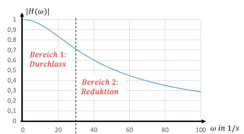
Magnitude of the transfer function |H(ω)| of a low-pass filter with ω_g = 30 1/s: pass band and attenuation range — Bereich = range · Durchlass = pass (passband) · Reduktion = reduction

\[ \begin{gathered} \text{Example: } \omega_g = 30\,\frac{1}{\mathrm{s}} \\[6pt] \text{General: } |H(\omega)| = \frac{1}{\sqrt{1 + (\omega RC)^2}} \\[6pt] \text{Range 1: } |H(\omega \ll \omega_g)| \approx \frac{1}{\sqrt{1}} = 1 \\[6pt] \text{At the cut-off frequency: } |H(\omega_g)| = \left|\frac{1}{\sqrt{1^2 + 1^2}}\right| = \frac{1}{\sqrt{2}} \approx 0.7 \\[6pt] \text{Range 2: } |H(\omega \gg \omega_g)| \approx \frac{1}{\sqrt{(\omega RC)^2}} = \frac{1}{\omega RC} \end{gathered} \]

How was the figure above created? We calculate the magnitude of the transfer function from |u_Aus / u_Ein| for many values of ω. We then plot these in the diagram with ω on the x-axis. Each value of the transfer function is valid for one signal frequency.

The cut-off frequency of the filter can be read from the figure above. At the cut-off frequency, the magnitude of the transfer function is |H(ω_g)| = 0.7.

The cut-off frequency of a system is set by the values of R and C in the circuit. So we can use the component values of the filter circuit to determine where the cut-off frequency lies. In the figure above I arbitrarily set it to ω_g = 30 1/s. You can choose other values by changing R and/or C. In general, we describe filters in the following form:

\[ \begin{gathered} |H| = \left|\frac{U_{\mathrm{Aus}}}{U_{\mathrm{Ein}}}\right| = \frac{1}{\sqrt{1 + (\omega RC)^2}} = \frac{1}{\sqrt{1 + (\omega/\omega_g)^2}} \\[6pt] \text{with } \omega_g = \frac{1}{RC} \end{gathered} \]