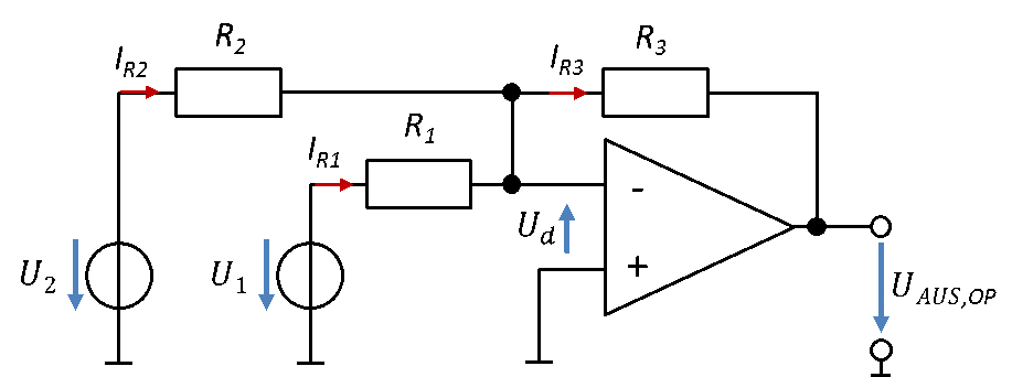
The summing amplifier is an op-amp circuit with two input voltage sources. One of the input sources is the sensor voltage. This is where you simply connect your sensor. The other is the shift voltage. You have to generate the shift voltage somewhere in your circuit. In the lab, you simply use a power supply for this. We will not look in more detail at how this voltage is generated.
First, I derive the transfer behaviour of the circuit. As a reminder: Ud = 0 V and no currents flow into the inputs of the op-amp. So we can set up the following equations:
The formula of the summing amplifier only applies if you set the values of the resistors R1 = R2 equal.
The mathematical operation in the brackets is carried out first. So this circuit first adds two voltages. Then it multiplies by the factor v. The gain v is negative, so the sum of the two signals is inverted once.
We cannot form a transfer function of the circuit. We can only do this with function blocks that have one input and one output. This circuit has two inputs. This is the case with every circuit that shifts and amplifies. It is not a problem; we can calculate the output voltage even without a transfer function.
This circuit is used as follows: since the gain is negative, the signal must be completely negative after shifting. A completely negative signal that is inverted by the gain is completely positive afterwards.
\[
\begin{gathered}
\text{Shifted signal purely negative: } u_S + U_V = [-x\,\mathrm{V} \ldots 0\,\mathrm{V}] \\[6pt]
\text{Negative gain } v\text{: minus times minus gives plus} \\[6pt]
(u_S + U_V) \cdot v = [0\,\mathrm{V} \ldots y\,\mathrm{V}] \text{ purely positive} \\[6pt]
\text{choose } v \text{ so that } U_{\mathrm{ADC,Max}} = U_{\mathrm{Ref}} \\[6pt]
v = \frac{y}{-x}
\end{gathered}
\]
Example
The sensor signal of the PT-100 on a current source with I0 = 10 mA lies in the range uS = [1 V … 1.4 V] over the measuring range T = [0 °C … 100 °C]. The reference voltage of the ADC is UREF,ADC = 3 V.
To adapt this signal to the ADC with a summing amplifier, we first have to make the signal completely negative. The upper limit should be 0 V. To do this, we have to add the shift voltage UV = −1.4 V to the sensor signal.
\[
\begin{gathered}
v = -\frac{R_3}{R_1} \rightarrow \text{e.g. } R_3 = 7.5\,\mathrm{k\Omega} \text{ and } R_1 = 1\,\mathrm{k\Omega} \\[6pt]
\text{Other pairs of values with the same ratio } v \text{ also work.}
\end{gathered}
\]
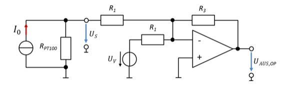
In the circuit above, the label R1 has been used twice for different resistors. This is meant to signal that the values of the resistors are equal. They are different resistors with equal values. This labelling is not common and not entirely clean, but it shows immediately that both values are equal.
The shift voltage is drawn as a voltage source. It can be implemented with a power supply, for example. The output of the sensor (PT-100 with current source) is connected where the other voltage source was used in the circuit diagram of the summing amplifier.
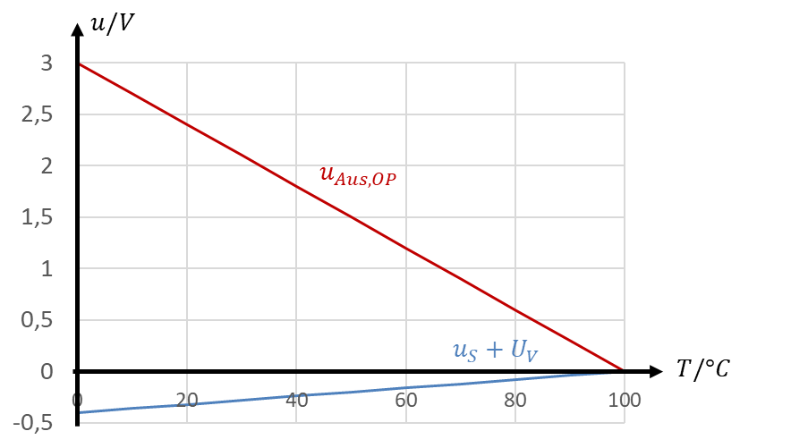
The characteristic of the output voltage of the op-amp versus temperature looks like this:
Aus = out (output)
The measuring range of the temperature now fits the input voltage range of the ADC optimally. The ADC digitises the voltage. In the example, we assume an 8-bit ADC.
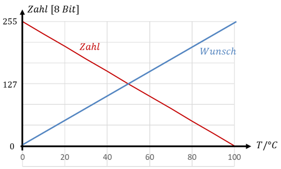
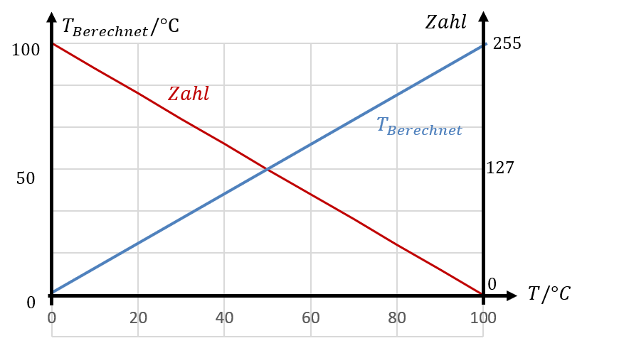
The characteristic of the numbers at the output of the ADC versus temperature is shown in red in the figure above. The characteristic has an offset and a slope error. Ideally, we would like the blue characteristic. We still have to carry out a digital correction in the digital signal processing.
The offset in the characteristic is the value at the temperature T = 0 °C. The offset number is 255. The offset is corrected by subtracting the offset number from all numbers output by the ADC. The slope is −255 / 100 °C. For an 8-bit ADC with UREF = 3 V, the following applies: