Electrical Engineering BMT & UFC › Alternating Current

Sine Mathematics

The sine function is used to calculate lengths and angles in a triangle. Let us look at a triangle with the side lengths a, b and c and the angle φ:

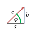
Right-angled triangle with hypotenuse c, opposite side b and angle φ

\[ \sin(\varphi) = \frac{b}{c} \]

In a triangle, the sine function gives the length of side b relative to the length of side c. We place this triangle in a circle in an x-y coordinate system:

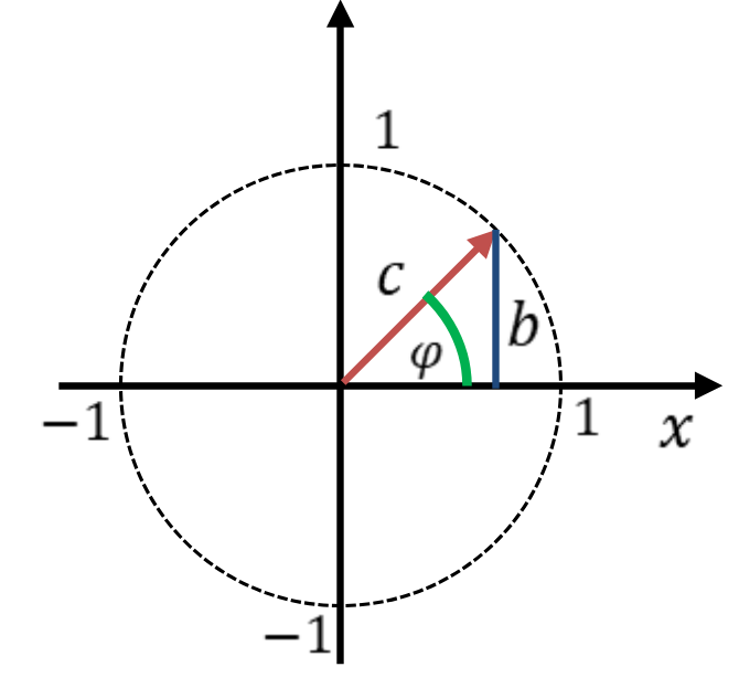
We mentally move the red pointer along the dashed black line in the figure above. This changes the angle φ, but we keep the length c of the red pointer constant. If the dashed circle always intersects the axes at the points 1 and −1, then c = 1 always applies. With c = 1, the relationship between b and c simplifies to:

\[ \begin{gathered} \sin(\varphi) = \frac{b}{c} \\[4pt] c = 1 \\[4pt] \sin(\varphi) = b \end{gathered} \]

This applies at all points of the dashed circle. The result of the sine function can be illustrated graphically on this circle. When the angle φ is changed, we can read off directly from the length of the blue line b how large the value of sin(φ) is. The sine of an angle can be read off from the length of a line. That is a good simplification.

If this is going too fast for you, I recommend the following video (in German) on the basics of sine and cosine:

Next, we increase the angle φ continuously over time. The red pointer thus moves anticlockwise around the circle. The following applies:

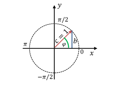
Unit circle with the angles 0, π/2, π and −π/2

\[ \begin{gathered} \varphi = 0 \ (3 \text{ o'clock})\text{: } b = 0 \\[4pt] \varphi = 90^\circ \text{ or } \varphi = \frac{\pi}{2} \ (12 \text{ o'clock})\text{: } b = 1 \\[4pt] \varphi = 180^\circ \text{ or } \varphi = \pi \ (9 \text{ o'clock})\text{: } b = 0 \\[4pt] \varphi = 270^\circ \text{ or } \varphi = \frac{3\pi}{2} \ (6 \text{ o'clock})\text{: } b = -1 \end{gathered} \]

The angle φ changes over the time t, and so the length b changes as well.

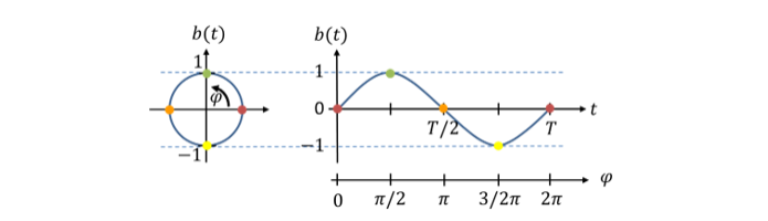
We define the time of one complete revolution as the period T. So T describes the time span until the curve repeats for the first time. At φ = 2π, t = T. The time t then equals one period T. Now we can transfer the curve of b onto a time axis and obtain the following graph for b(t):

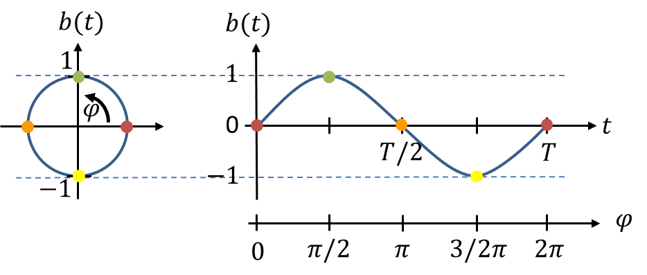
Revolution on the unit circle and the associated sine curve b(t)

The coloured points on the circle correspond to those in the time curve on the right. The y-values, i.e. the values of b(t), match on the left and right. One complete revolution of the circle – i.e. one period – is shown. The angle φ has the range of values φ = [0 .. 2π].

The curve b(t) = sin(φ) does not yet show any dependence on time. If the angle changes over time, we need a formula for its time dependence. The following applies:

\[ \begin{gathered} \varphi = \frac{2\pi}{T} \cdot t \\[6pt] b(t) = \sin\left(2\pi \cdot \frac{t}{T}\right) \end{gathered} \]

To check whether this formula correctly reproduces the curve in the right-hand figure, we substitute a few values for t as a test. Over one revolution, the time t changes in the range t = [0 .. T].

Unit circle and sine curve with marked points

\[ \begin{gathered} \text{Red point: } t = 0\text{: } b(0\,\mathrm{s}) = \sin(0) = 0 \\[6pt] \text{Green point: } t = \frac{T}{4}\text{: } b\left(\frac{T}{4}\right) = \sin\left(2\pi \cdot \frac{T/4}{T}\right) = \sin\left(\frac{\pi}{2}\right) = 1 \\[6pt] \text{Orange point: } t = \frac{T}{2}\text{: } b\left(\frac{T}{2}\right) = \sin\left(2\pi \cdot \frac{T/2}{T}\right) = \sin(\pi) = 0 \\[6pt] \text{Yellow point: } t = \frac{3T}{4}\text{: } b\left(\frac{3T}{4}\right) = \sin\left(2\pi \cdot \frac{3T/4}{T}\right) = \sin\left(\frac{3}{2}\pi\right) = -1 \\[6pt] \text{Red point: } t = T\text{: } b(T) = \sin\left(2\pi \cdot \frac{T}{T}\right) = \sin(2\pi) = 0 \end{gathered} \]

By substituting numerical values into a formula, we have shown that this formula is valid. All the numerical values correspond to the expected values that we see in the graph of the circle.

We can also substitute values of t outside the period T into the formula. Then we turn the point around the circle once and then further. We can also omit every complete revolution without changing the result. For example, sin(3π) = sin(π). A complete revolution has the angle 2π. So a rotation by 3π turns once around the circle and then by π further.

We have thus found a formula with which we can mathematically describe quantities that keep rotating on a circle. These are sinusoidal quantities of the general form

\[ b(t) = \sin\left(\frac{2\pi}{T} \cdot t\right) \]

The parameter t in the equation represents time. It is like the x in equations with f(x) in school mathematics. If you want to calculate b at a certain time, you substitute this time t into the equation. The formula then has a single solution b as a number. But that is not what we want to achieve at all. The formula itself is the solution to the problem: the mathematical description of an AC quantity over the time t. So you normally do not substitute a time value for t; instead, you use this formula for further calculations.

It is like a straight-line equation y = m ∙ x + b, for example. The equation describes all points y on the straight line mathematically. You can calculate a value y by substituting x. That is nice, but often not the goal. You can also use the equation to check whether another straight line runs parallel to it or intersects it. For this, you need the equation itself, not a single numerical value. In electrical engineering, we use the equation above for further calculations.