Pole Compensation

Most real systems contain several integrating or delaying components. These increase the tendency to oscillate and slow the system down. Differentiating behaviour speeds the system up. It is therefore an obvious idea to use D behaviour to compensate specifically for unwanted I behaviour. We have:

\[ \begin{gathered} \text{I behaviour: } \frac{1}{s} \\[6pt] \text{D behaviour: } s \\[6pt] \text{Combination: } s \cdot \frac{1}{s} = 1 \end{gathered} \]

Unfortunately, the terms often do not appear as pure I behaviour but rather as PT-1 behaviour. Then:

\[ \begin{gathered} \text{PT1 behaviour: } \frac{1}{1 + \tau s} \\[6pt] \text{Compensation: } 1 + \tau s \\[6pt] \text{Combination: } (1 + \tau s) \cdot \frac{1}{1 + \tau s} = 1 \end{gathered} \]

Before we deal with compensation, let us first look at the behaviour of an example system with I behaviour and PT-1 behaviour. First, a pure P controller is used without compensating for any behaviour.

Simulation model: step w, PID controller, integrator 1/s and PT1 plant 1/(s + 1) with oscilloscope

\[ \begin{gathered} \text{Pure P controller: } k_{PR} = 1,\ k_{IR} = 0,\ k_{DR} = 0 \\[6pt] A = \frac{k_{PR}}{s^2 + s} = \frac{1}{s^2 + s} \rightarrow \frac{1}{A} = s^2 + s \rightarrow H_{\mathrm{FÜ}} = \frac{1}{s^2 + s + 1} \\[6pt] \text{Comparing coefficients: } \frac{1}{\omega_0^2} = 1 \rightarrow \omega_0 = 1\,\frac{1}{\mathrm{s}} \rightarrow f_0 = 0.16\,\mathrm{Hz} \rightarrow T = 6.28\,\mathrm{s} \\[6pt] \frac{2D}{\omega_0} = 1 \rightarrow D = 0.5\text{, decaying oscillation} \end{gathered} \]

Simulated step response with a pure P controller: decaying oscillation around the setpoint

(H_FÜ: reference transfer function.)

Compensating the PT-1 behaviour of the plant

In the first step, the PT-1 behaviour of the plant (far right) is to be compensated by a suitable choice of controller:

\[ \begin{gathered} A = H_{\mathrm{PID}} \cdot \frac{1}{s} \cdot \frac{1}{1 + s} \\[6pt] \text{Goal: } H_{\mathrm{PID}} = 1 + s \\[6pt] A = (1 + s) \cdot \frac{1}{s} \cdot \frac{1}{1 + s} = \frac{1}{s} \\[6pt] H_{\mathrm{FÜ}} = \frac{1}{1 + \frac{1}{A}} = \frac{1}{1 + s} \\[6pt] \text{Controlled system with PT1 behaviour with } \tau = 1 \end{gathered} \]

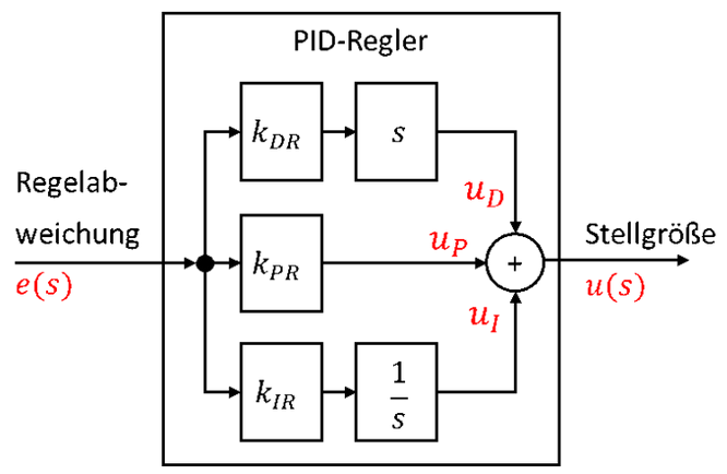
Question: How can the compensation term 1 + s be generated with a PID controller? To answer this, let us look again at the structure of a PID controller:

PID controller in the frequency domain: parallel connection of D part (k_DR, s), P part (k_PR) and I part (k_IR, 1/s) — PID-Regler = PID controller · Regelabweichung = control error · Stellgröße = manipulated variable

The PID controller adds the P, I and D parts at its output. This leads to the following transfer function:

\[ \begin{gathered} H_{\mathrm{PID}} = \frac{u(s)}{e(s)} = k_{PR} + k_{IR} \cdot \frac{1}{s} + k_{DR} \cdot s \\[6pt] \text{Goal: } H_{\mathrm{PID}} = 1 + s \rightarrow k_{PR} = 1,\ k_{IR} = 0 \text{ and } k_{DR} = 1 \end{gathered} \]

Overall, this controller produces the desired behaviour. Here is the calculation once more in summary:

\[ \begin{gathered} A = H_{\mathrm{PID}} \cdot \frac{1}{s} \cdot \frac{1}{1 + s} \\[6pt] \text{with } k_{PR} = 1,\ k_{IR} = 0 \text{ and } k_{DR} = 1 \text{ it follows that} \\[6pt] H_{\mathrm{PID}} = 1 + s \\[6pt] A = (1 + s) \cdot \frac{1}{s} \cdot \frac{1}{1 + s} = \frac{1}{s} \\[6pt] H_{\mathrm{FÜ}} = \frac{1}{1 + \frac{1}{A}} = \frac{1}{1 + s} \\[6pt] \text{PT1 behaviour with } \tau = 1 \end{gathered} \]

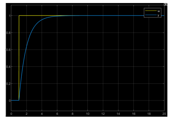
Simulated step response with pole compensation: PT1 curve with τ = 1

The step response of the controlled system shows that only PT-1 behaviour remains. With correctly dimensioned P and D parts, the PID controller was able to compensate exactly for a PT-1 behaviour in the plant. The system then behaves as if A contained only pure I behaviour.

Compensating the I behaviour of the plant

Next, we try to remove the pure I behaviour from the plant. Then only PT-1 behaviour should remain in A.

\[ \begin{gathered} A = H_{\mathrm{PID}} \cdot \frac{1}{s} \cdot \frac{1}{1 + s} \\[6pt] \text{with } k_{PR} = 0,\ k_{IR} = 0 \text{ and } k_{DR} = 1 \text{ it follows that} \\[6pt] H_{\mathrm{PID}} = s \\[6pt] A = s \cdot \frac{1}{s} \cdot \frac{1}{1 + s} = \frac{1}{1 + s} \\[6pt] H_{\mathrm{FÜ}} = \frac{1}{1 + \frac{1}{A}} = \frac{1}{1 + s + 1} = \frac{1}{2 + s} = \frac{0.5}{1 + 0.5\,s} \\[6pt] \text{PT1 behaviour with } \tau = 0.5 \end{gathered} \]

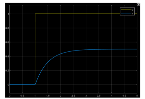
Simulated step response with k_PR = 0: PT1 curve with τ = 0.5 and final value 0.5

Using a pure D controller, we have succeeded in ideally compensating for the pure I behaviour of the plant.

Faulty compensation

To apply this method, the system must have been measured and modelled very accurately. For PT-1 behaviour, τ must be known and must not change. The method works very well in theory; in practice its use is more difficult, because the system parameters change due to ageing, wear, temperature or non-linear system behaviour. Compensation can only work with exact knowledge of the parameters.

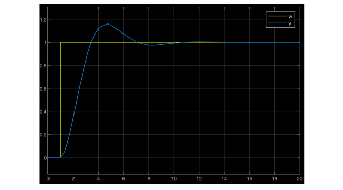
To demonstrate practical problems, the example system is compensated with a wrongly configured controller. Again we try to compensate for the PT-1 behaviour of the plant:

\[ \begin{gathered} A = H_{\mathrm{PID}} \cdot \frac{1}{s} \cdot \frac{1}{1 + s} \\[6pt] \text{with } k_{PR} = \mathbf{2}\ \textbf{(wrong!)},\ k_{IR} = 0 \text{ and } k_{DR} = 1 \text{ it follows that} \\[6pt] H_{\mathrm{PID}} = \mathbf{2} + s \\[6pt] A = (\mathbf{2} + s) \cdot \frac{1}{s} \cdot \frac{1}{1 + s} = \frac{(\mathbf{2} + s)}{s \cdot (1 + s)} \\[6pt] H_{\mathrm{FÜ}} = (\ldots) = \frac{2 + s}{s^2 + 2s + 2} \end{gathered} \]

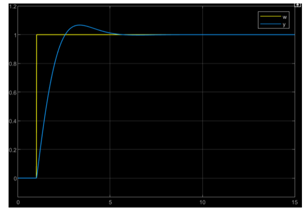
Simulated step response with wrongly chosen k_PR = 2: slight overshoot

With incorrect compensation, the system again shows PT-2 behaviour with overshoot. A more detailed discussion of polynomials in the numerator and denominator of the reference transfer function goes beyond the scope of this lecture.

End