Learning Content and Theses

Platform for digital learning at HSHL

High-Pass Filter

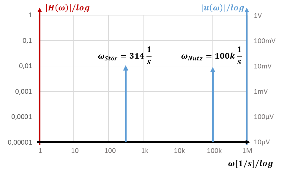
A high-pass filter lets high-frequency signals pass and attenuates low-frequency signals. As an example, let us take a typical low-frequency interference: mains hum at fNetz = 50 Hz. All measurement systems connected to the 230 V mains have an interference signal with a small amplitude at 50 Hz in the measurement signal. For the example, let us assume that a useful signal has the frequency ωNutz = 100k 1/s. The angular frequency of the interference is ωStör = 2πfNetz = 314 1/s. Peak values and frequencies are shown in the Bode plot below (Netz = mains, Nutz = useful, Stör = interference).

The peak value of the interference signal should be reduced as much as possible by a filter; the useful signal should not be affected by the filter. The two signals are again shown as arrows in the frequency domain.

Spectrum with interference signal at ω_Stör = 314 1/s and useful signal at ω_Nutz = 100k 1/s
Stör = disturbance · Nutz = useful

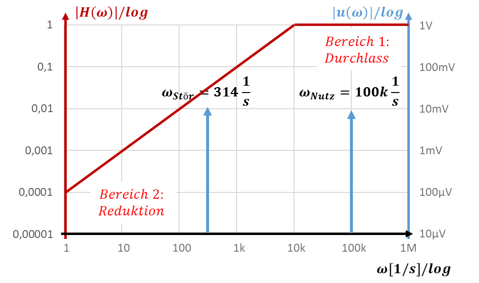
A suitable filter leaves the useful signal unchanged by having a horizontal curve with |H| = 1 at the useful signal. The nearest cut-off frequency is a factor of 10 away from the useful signal; otherwise the filter already has too much influence on the useful signal (see the discussion in the chapter on the low-pass filter). It attenuates the interference signal; the magnitude of its transfer function at ωStör is less than 1. This is described by the following desired Bode plot of a filter:

Bode approximation of a high-pass filter with ω_g = 10k 1/s: attenuation below, pass band above the cut-off frequency
Bereich = range · Reduktion = reduction · Durchlass = pass (passband) · Nutz = useful

From the diagram we read that the interference signal is amplified by the filter by a factor of about 0.03. So it is attenuated by a factor of about 30. This behaviour is called “high-pass” because it lets signals of high frequencies pass and attenuates signals of low frequencies.

Implementation and dimensioning

First, a passive implementation without an operational amplifier is discussed. For cost reasons, the solution again uses a capacitor instead of an inductor. The simplest high-pass filter is built from the series connection of a capacitor and a resistor. We first look at the derivation with complex numbers, further down at the one with reactances:

Derivation with complex numbers

RC high-pass filter: capacitor C in series, resistor R at the output
Aus = out (output)
\[ \underline{H}_{\mathrm{Filter}}(\omega) = \frac{\underline{u}_{\mathrm{Aus}}}{\underline{u}_{\mathrm{Ein}}} = \frac{\underline{Z}_R}{\underline{Z}_R + \underline{Z}_C} = \frac{R}{R + \frac{1}{j\omega C}} = \frac{j\omega RC}{1 + j\omega RC} = \frac{j\omega/\omega_g}{1 + j\omega/\omega_g} \text{ with } \omega_g = \frac{1}{RC} \]

In the last conversion step, I expanded the fraction by jωC. First, let us again look at the two ranges of the transfer function:

\[ \begin{gathered} \underline{H}_{\mathrm{Filter}}(\omega) = \frac{j\omega/\omega_g}{1 + j\omega/\omega_g} \end{gathered} \]
\[ \begin{gathered} \text{Range 1: } \omega \ll \omega_g \\[6pt] \text{This range includes } \omega = 0\,\tfrac{1}{\mathrm{s}}\text{: } \underline{H}_{\mathrm{Filter}}\left(0\,\tfrac{1}{\mathrm{s}}\right) = \frac{j0/\omega_g}{1 + j0/\omega_g} = 0 \\[6pt] \text{In the denominator: } 1 \gg j\omega/\omega_g \\[6pt] \underline{H}_{\mathrm{Filter}}(\omega) = \frac{j\omega/\omega_g}{1 + j\omega/\omega_g} \approx \frac{j\omega/\omega_g}{1} \sim \omega \\[6pt] \text{The transfer function increases linearly with increasing } \omega. \end{gathered} \]
\[ \begin{gathered} \text{Range 2: } \omega \gg \omega_g \\[6pt] \text{This range includes } \omega \rightarrow \infty\text{: } \underline{H}_{\mathrm{Filter}}(\infty) = \frac{j\infty/\omega_g}{1 + j\infty/\omega_g} = 1 \\[6pt] \text{In the denominator: } 1 \ll j\omega/\omega_g \\[6pt] \underline{H}_{\mathrm{Filter}}(\omega) = \frac{j\omega/\omega_g}{1 + j\omega/\omega_g} \approx \frac{j\omega/\omega_g}{j\omega/\omega_g} = 1 \\[6pt] \text{The transfer function is constant.} \end{gathered} \]

The behaviour of the Bode plot matches the transfer function of the circuit. So this circuit implements (passive) high-pass behaviour. Again we only consider the magnitude of the transfer function. The following applies:

\[ |\underline{H}_{\mathrm{Filter}}(\omega)| = \left|\frac{j\omega/\omega_g}{1 + j\omega/\omega_g}\right| = \frac{\omega/\omega_g}{\sqrt{1 + \omega^2/\omega_g^2}} \]

Derivation with reactances

RC high-pass filter: capacitor C in series, resistor R at the output
Aus = out (output)
\[ H_{\mathrm{Filter}}(\omega) = \frac{\hat{u}_{\mathrm{Aus}}}{\hat{u}_{\mathrm{Ein}}} = \frac{R}{\sqrt{R^2 + X_C^2}} = \frac{R}{\sqrt{R^2 + \frac{1}{\omega^2 C^2}}} = \frac{\omega RC}{\sqrt{1 + R^2 \omega^2 C^2}} = \frac{\omega/\omega_g}{\sqrt{1 + \omega^2/\omega_g^2}} \text{ with } \omega_g = \frac{1}{RC} \]

First, let us again look at the two ranges of the transfer function:

\[ H_{\mathrm{Filter}}(\omega) = \frac{\omega/\omega_g}{\sqrt{1 + \omega^2/\omega_g^2}} \]
\[ \begin{gathered} \text{Range 1: } \omega \ll \omega_g \\[6pt] \text{This range includes } \omega = 0\,\tfrac{1}{\mathrm{s}}\text{: } H_{\mathrm{Filter}}\left(0\,\tfrac{1}{\mathrm{s}}\right) = \frac{0/\omega_g}{\sqrt{1 + 0^2/\omega_g^2}} = 0 \\[6pt] \text{In the denominator: } 1^2 \gg \left(\frac{\omega}{\omega_g}\right)^2 \\[6pt] H_{\mathrm{Filter}}(\omega) = \frac{\omega/\omega_g}{\sqrt{1 + \omega^2/\omega_g^2}} \approx \frac{\omega/\omega_g}{1} \sim \omega \\[6pt] \text{The transfer function increases linearly with increasing } \omega. \end{gathered} \]
\[ \begin{gathered} \text{Range 2: } \omega \gg \omega_g \\[6pt] \text{This range includes } \omega \rightarrow \infty\text{: } H_{\mathrm{Filter}}(\infty) = \frac{\infty/\omega_g}{\sqrt{1 + \infty^2/\omega_g^2}} = 1 \\[6pt] \text{In the denominator: } 1^2 \ll \left(\frac{\omega}{\omega_g}\right)^2 \\[6pt] H_{\mathrm{Filter}}(\omega) = \frac{\omega/\omega_g}{\sqrt{1 + \omega^2/\omega_g^2}} \approx \frac{\omega/\omega_g}{\omega/\omega_g} = 1 \\[6pt] \text{The transfer function is constant.} \end{gathered} \]

Again we only consider the magnitude of the transfer function. The following applies:

\[ |H_{\mathrm{Filter}}(\omega)| = \frac{\omega/\omega_g}{\sqrt{1 + \omega^2/\omega_g^2}} \]

High-pass filter with inductor and resistor

Note: this subchapter is not relevant for the exam. It is explained with complex numbers only.

I mentioned in previous chapters that filters can also be implemented with inductors. I would like to show this once with a high-pass filter. In measurement practice we tend to use capacitors, because they are cheaper and smaller, and inductors disturb other parts of the circuit with their field.

All circuits whose transfer function shows high-pass behaviour also act as a high-pass filter. So we are looking for a circuit with an inductor and a resistor that shows the following behaviour:

\[ \text{General transfer function of a high-pass filter: } H = \frac{j\frac{\omega}{\omega_g}}{1 + j\frac{\omega}{\omega_g}} \]
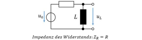
Series connection of resistor R and inductor L, output u_L across the inductor
Impedanz = impedance · Widerstand = resistor
\[ \begin{gathered} \text{Impedance of the resistor: } \underline{Z}_R = R \\[6pt] \text{Impedance of the inductor: } \underline{Z}_L = j\omega L \\[6pt] \text{Voltage divider: } \underline{u}_L = \underline{u}_0 \cdot \frac{\underline{Z}_L}{\underline{Z}_R + \underline{Z}_L} = \underline{u}_0 \cdot \frac{j\omega L}{R + j\omega L} \\[6pt] \text{Divide by } R\text{: } \underline{u}_L = \underline{u}_0 \cdot \frac{j\omega\frac{L}{R}}{1 + j\omega\frac{L}{R}} = \underline{u}_0 \cdot \frac{j\frac{\omega}{\omega_0}}{1 + j\frac{\omega}{\omega_0}} \text{ with } \omega_0 = \frac{R}{L} \\[6pt] \underline{H} = \frac{\underline{u}_L}{\underline{u}_0} = \frac{j\frac{\omega}{\omega_0}}{1 + j\frac{\omega}{\omega_0}} \rightarrow \text{high-pass behaviour} \end{gathered} \]

Inductors and capacitors behave reciprocally in many respects. If you build a low-pass filter from a resistor and a capacitor and replace the capacitor with an inductor, you obtain a high-pass filter.

Choosing the cut-off frequency

Note: from here on, the content is relevant for the exam again.

The cut-off frequency must be placed so that the useful signal passes the filter almost unchanged and the interference is attenuated as much as possible. For the high-pass filter, we therefore place the cut-off frequency a factor of 10 below the useful frequency. Caution: for the low-pass filter it is exactly the other way round!

\[ \begin{gathered} \omega_g = 0.1 \cdot \omega_{\mathrm{Nutz}} \\[6pt] f_g = 0.1 \cdot f_{\mathrm{Nutz}} \end{gathered} \]

Active high-pass filter

All circuits whose transfer function can be transformed into the term

\[ |H_{\mathrm{Filter}}(\omega)| = \frac{\omega/\omega_g}{\sqrt{1 + \omega^2/\omega_g^2}} \]

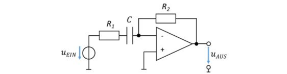
are high-pass filters. This behaviour is achieved in the following amplifier circuit:

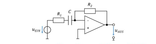
Active high-pass filter: R_1 and C in series before the inverting amplifier, feedback via R_2
Ein = in (input)
\[ \begin{gathered} \textcolor{#c00000}{\text{Complex numbers: } \underline{H}(\omega) = -\frac{\underline{Z}_2}{\underline{Z}_1} = -\frac{R_2}{R_1 + \frac{1}{j\omega C}} = -\frac{j\omega R_2 C}{1 + j\omega R_1 C} = -\frac{j\omega R_1 R_2 C}{R_1(1 + j\omega R_1 C)}} \\[6pt] \textcolor{#c00000}{= -\frac{R_2}{R_1} \cdot \left(\frac{j\omega R_1 C}{1 + j\omega R_1 C}\right) = v \cdot \left(\frac{\frac{j\omega}{\omega_g}}{1 + \frac{j\omega}{\omega_g}}\right) \rightarrow |\underline{H}(\omega)| = |v| \cdot \left(\frac{\omega/\omega_g}{\sqrt{1 + \omega^2/\omega_g^2}}\right)} \end{gathered} \]
\[ \begin{gathered} \textcolor{#1f5fbf}{\text{Reactances: } H(\omega) = -\frac{X_2}{X_1} = -\frac{R_2}{\sqrt{R_1^2 + \frac{1}{\omega^2 C^2}}} = -\frac{\omega R_2 C}{\sqrt{1 + R_1^2 \omega^2 C^2}} = -\frac{R_1 \cdot \omega R_2 C}{R_1 \cdot \sqrt{1 + R_1^2 \omega^2 C^2}}} \\[6pt] \textcolor{#1f5fbf}{= -\frac{R_2}{R_1} \cdot \frac{\omega R_1 C}{\sqrt{1 + R_1^2 \omega^2 C^2}} = v \cdot \left(\frac{\omega/\omega_g}{\sqrt{1 + \omega^2/\omega_g^2}}\right) \rightarrow |H(\omega)| = |v| \cdot \left(\frac{\omega/\omega_g}{\sqrt{1 + \omega^2/\omega_g^2}}\right)} \end{gathered} \]

Now you can see a term for the frequency-independent gain v = −R2/R1 and the filter with the cut-off frequency ωg = 1/(R1C). The circuit structure implements amplification and high-pass filtering. The amount of gain and the cut-off frequency of the filter are determined by the component values, which you set specifically for your application.

Remember: in this circuit, the components between the voltage source and the inverting input determine the cut-off frequency. In the series connection it does not matter whether the capacitor is placed to the left or right of resistor R1.

Task

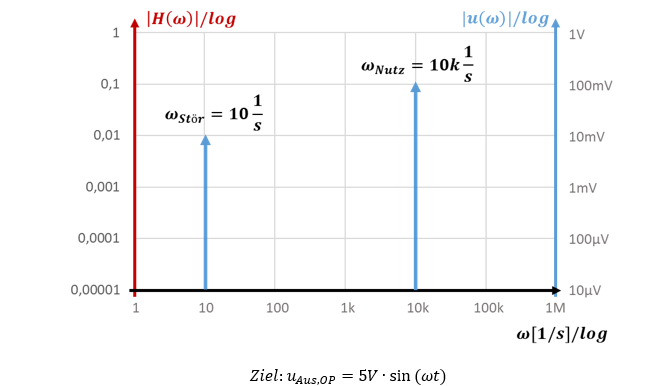
Spectrum of the task: interference signal at 10 1/s, useful signal at 10k 1/s
Nutz = useful · Ziel = target · Aus = out (output) · Stör = disturbance
\[ \begin{gathered} \text{Goal: } u_{\mathrm{Aus,OP}} = 5\,\mathrm{V} \cdot \sin(\omega t) \\[6pt] u_{\mathrm{Sensor}} = u_{\mathrm{Nutz}} + u_{\mathrm{Stör}} \\[6pt] u_{\mathrm{Nutz}} = 100\,\mathrm{mV} \cdot \sin(\omega_{\mathrm{Nutz}} t) \text{ with } \omega_{\mathrm{Nutz}} = 10\mathrm{k}\,\tfrac{1}{\mathrm{s}} \\[6pt] u_{\mathrm{Stör}} = 10\,\mathrm{mV} \cdot \sin(\omega_{\mathrm{Stör}} t) \text{ with } \omega_{\mathrm{Stör}} = 10\,\tfrac{1}{\mathrm{s}} \end{gathered} \]

Tasks:

  • Determine the circuit structure, filter type, cut-off frequency and gain
  • Dimension the components. \(R_1 = 1\,\mathrm{k\Omega}\) applies.
  • By what factor does the circuit increase the signal-to-noise ratio?

Solution

The gain is designed for the useful signal. 100 mV must be amplified to 5 V; for this we need a factor of 50. So we need an amplifier and not a passive solution. The gain of the inverting amplifier for filters is then v = −50. The sign does not matter for sinusoidal quantities; it only rotates the phase by 180°.

The interference frequency is lower than the useful frequency, so we need an (active) high-pass filter. For a high-pass filter, the cut-off frequency is placed a factor of 10 below the useful frequency, in this example at 1k 1/s.

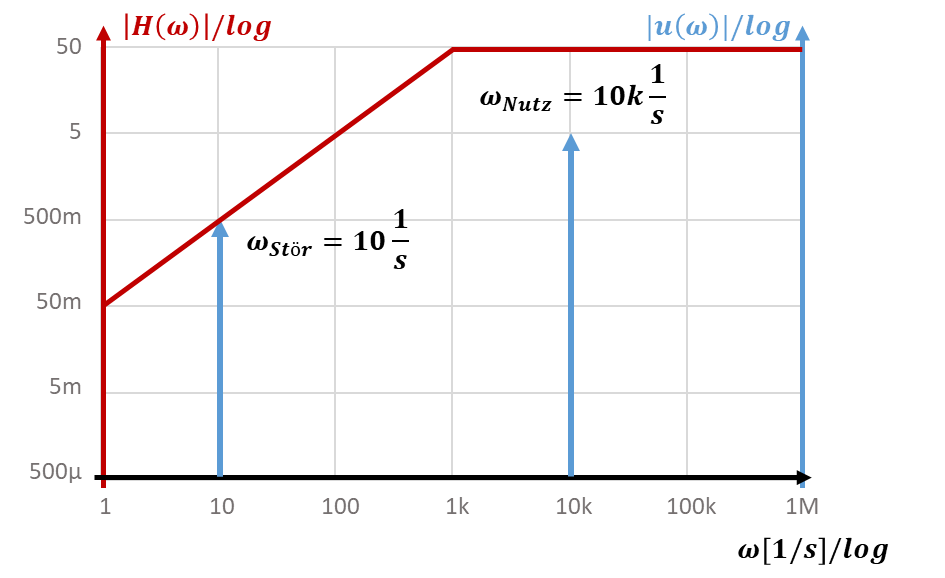
With this we move on to dimensioning. I draw the Bode plot directly for the whole circuit, i.e. I include the gain of v = −50 (caution: magnitude!) in the left-hand axis:
Bode plot of the solution: high-pass filter with ω_g = 1k 1/s and gain 50
Active high-pass filter of the solution
Aus = out (output)
\[ \begin{gathered} |H(\omega)| = |v| \cdot \left(\frac{\omega/\omega_g}{\sqrt{1 + \omega^2/\omega_g^2}}\right) = \left|-\frac{R_2}{R_1}\right| \cdot \left(\frac{\omega/\omega_g}{\sqrt{1 + \omega^2/\omega_g^2}}\right) \text{ with } \omega_g = \frac{1}{R_1 C} \\[6pt] v = -50 = -\frac{R_2}{R_1} \rightarrow R_2 = 50 \cdot R_1 = 50 \cdot 1\,\mathrm{k\Omega} = 50\,\mathrm{k\Omega} \\[6pt] \omega_g = 1\mathrm{k}\,\frac{1}{\mathrm{s}} = \frac{1}{R_1 C} \rightarrow C = \frac{1}{R_1 \omega_g} = \frac{1}{1\,\mathrm{k\Omega} \cdot 1\mathrm{k}\,1/\mathrm{s}} = 1\,\text{µF} \\[6pt] u_{\mathrm{Nutz}}(\omega) = 100\,\mathrm{mV};\ u_{\mathrm{Stör}}(\omega) = 10\,\mathrm{mV} \\[6pt] |u_{\mathrm{Aus,OP,Nutz}}| = |H(\omega_{\mathrm{Nutz}})| \cdot u_{\mathrm{Nutz}}(\omega) = 50 \cdot 100\,\mathrm{mV} = 5\,\mathrm{V} \\[6pt] |u_{\mathrm{Aus,OP,Stör}}| = |H(\omega_{\mathrm{Stör}})| \cdot u_{\mathrm{Stör}}(\omega) = 0.5 \cdot 10\,\mathrm{mV} = 5\,\mathrm{mV} \\[6pt] \text{SNR at the op-amp input: } \mathrm{SSA}_{\mathrm{Ein}} = \left|\frac{u_{\mathrm{Nutz}}}{u_{\mathrm{Stör}}}\right| = \frac{100\,\mathrm{mV}}{10\,\mathrm{mV}} = 10 \\[6pt] \text{SNR at the op-amp output: } \mathrm{SSA}_{\mathrm{Aus}} = \left|\frac{u_{\mathrm{Aus,OP,Nutz}}}{u_{\mathrm{Aus,OP,Stör}}}\right| = \frac{5\,\mathrm{V}}{5\,\mathrm{mV}} = 1000 \end{gathered} \]

Simulation

The circuit increases the signal-to-noise ratio from 10 to 1000, i.e. by a factor of 100.

Download course as PDF

The PDF contains all pages of the course. Interactive content is only available on the website.