Control Engineering › System Behaviors 1

PT1 Behavior

If a storage element is filled via a block with proportional behaviour, we call this PT behaviour in control engineering. One example is “filling” a capacitor via a resistor in electrical engineering. This is explained with the water model in this chapter. Please read that chapter before continuing here.

There is PT behaviour of different orders. The more storage elements in the system are charged and discharged, the higher the order. A PT1 system has one storage element, a PT2 system has 2 storage elements, and so on. Energy storage elements make a system sluggish, which is why a system with many storage elements and thus a high order generally reacts slowly.

Optional: transfer function in the time domain

The transfer function of a system with PT1 behaviour is mathematically complicated to derive and calculate. So the following text is not only about PT1 behaviour. It is also about how we deal with (too) difficult mathematics. I show you ways of simplifying complicated mathematics in general and verifying formulas that you do not understand.

This subchapter “Transfer function in the time domain” is not relevant for the control engineering exam. It is aimed at interested students who want to improve their ability to handle complex mathematics. Lean back and, for a change, enjoy a text that will never be examined. At the end of the chapter, it becomes relevant for the exam again.

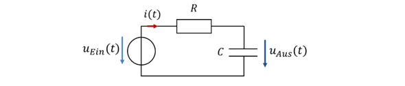
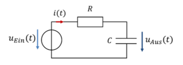
The derivation of PT1 behaviour uses an example whose solution we already know from the fundamentals of electrical engineering. This makes it easy to verify the result at the end of the derivation. We look at a series connection of a resistor (P behaviour) with a capacitor (I behaviour) on a voltage source. The input quantity is the source voltage. The output quantity is the capacitor voltage. As usual in control engineering, we look at the step response of the system to characterise its properties. So we apply a step in the input voltage from 0 V to 1 V and look at the output voltage. The following applies:

RC element: voltage source u_Ein(t), resistor R, capacitor C with output voltage u_Aus(t) — Ein = in (input)

\[ \begin{gathered} \text{Specific solution for the example from electrical engineering:} \\[6pt] \text{Mesh equation: } u_{\mathrm{Ein}}(t) = u_R(t) + u_C(t) \\[6pt] \text{Component equations: } u_R(t) = R \cdot i(t) \text{ and } u_C(t) = \frac{1}{C} \cdot \int i(t)\,dt + u_{C0} \\[6pt] \text{Substitute: } u_{\mathrm{Ein}}(t) = R \cdot i(t) + \frac{1}{C} \cdot \int i(t)\,dt + u_{C0} \\[6pt] u_{\mathrm{Aus}}(t) = u_C(t) \end{gathered} \]

The equation is an integral equation (after differentiating, a differential equation). The term i(t) and the integral of i(t) appear in one equation. You have (probably) not yet learned the mathematics to solve this equation for u_Aus(t). So I simply give you the solution of this equation in the time domain, and we analyse it at characteristic points.

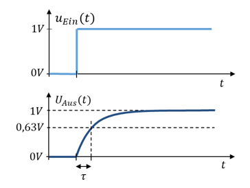
\[ \begin{gathered} i(t) = \frac{u_{\mathrm{Ein}}(t)}{R} \cdot e^{-\frac{t}{\tau}} \text{ with } \tau = RC \\[6pt] u_{\mathrm{Aus}}(t) = u_{\mathrm{Ein}}(t) \left(1 - e^{-\frac{t}{\tau}}\right) \\[6pt] H(t) = \frac{u_{\mathrm{Aus}}(t)}{u_{\mathrm{Ein}}(t)} = 1 - e^{-\frac{t}{\tau}} \end{gathered} \]

Step of u_Ein(t) to 1 V and rise of u_Aus(t) with time constant τ to 0.63 V

The time curves of input and output voltage are known from the fundamentals of electrical engineering. It would not surprise me if you cannot do anything with them. How much does an equation really help in understanding a behaviour? We should insert values into the equation to understand how the system behaves at certain points in time. The moment of the step in the input voltage (t = 0 s) and the steady state as t tends to infinity are obvious choices.

Step response of the RC element at the step time t = 0 s and for t → ∞ — Ein = in (input)

\[ \begin{gathered} \text{Step time } t = 0\,\mathrm{s}\text{:} \\[6pt] H(0\,\mathrm{s}) = 1 - e^{-\frac{0\,\mathrm{s}}{\tau}} = 1 - 1 = 0 \\[6pt] u_{\mathrm{Aus}}(0\,\mathrm{s}) = H(0\,\mathrm{s}) \cdot u_{\mathrm{Ein}}(0\,\mathrm{s}) = 0 \cdot 1\,\mathrm{V} = 0\,\mathrm{V} \end{gathered} \]

\[ \begin{gathered} \text{Steady state: } t \rightarrow \infty\text{:} \\[6pt] H(\infty) = 1 - e^{-\frac{\infty}{\tau}} = 1 - 0 = 1 \\[6pt] u_{\mathrm{Aus}}(\infty) = H(\infty) \cdot u_{\mathrm{Ein}}(\infty) = 1 \cdot 1\,\mathrm{V} = 1\,\mathrm{V} \end{gathered} \]

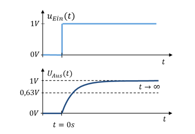
At both points in time, we obtain by calculation the result for the output voltage that can also be seen in the graph of the time curve. That is a good start. In addition, we need a handle on the formula that gives us a feel for the behaviour over time. The parameter τ is suitable for this.

The parameter τ = RC corresponds to the time between the start of the step in the input voltage and the moment at which the output voltage reaches 63 % of its final value. The parameter τ is characteristic of the behaviour of the system. If τ is large, the output voltage takes longer to reach the final value; the curve is flatter. If τ is small, the output voltage rises faster. The rise is always an exponential function. From τ we can directly infer the behaviour of the system between the step time and the steady state.

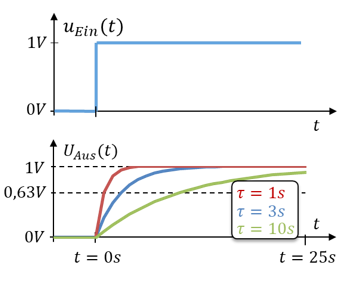
Step responses of the RC element for τ = 1 s, 3 s and 10 s — Aus = out (output)

Now we could take a set-up with a resistor and a capacitor and measure how long the output voltage takes after a step in the input voltage to reach 63 % of its final value. This time corresponds to τ. If the measured values agree with the mathematics, the equation solves the problem described. If not, you have to keep looking for the right solution.

It is easier in a simulation. Simulate the problem, e.g. in Multisim, and check the result at certain points in time t.

In general: if you cannot solve a problem mathematically, you can look up the solution. But then you absolutely must check that it is correct. It is a good idea to use an example for which you already know the result. You can use it to check whether the formula you found is actually correct.

To do so, insert numerical values at points where the result is known. Usually 0 and infinity are suitable. Perhaps you can find other suitable numbers. You verify whether the results of the formula you found match your expectations. If they do, it is highly likely that the formula actually describes your problem mathematically.

Transfer function in the frequency domain

From here on, the text is relevant for the exam again. Calculation in the time domain with differential equations, integral calculus and exponential functions is complicated. That is why we use the Laplace transform to solve the equation. We do this with every differential equation. The following applies:

\[ \begin{gathered} \text{Laplace transform:} \\[6pt] u_{\mathrm{Ein}}(\omega) = u_R(\omega) + u_C(\omega) \\[6pt] u_R(\omega) = R \cdot i(\omega) \text{ and } u_C(\omega) = \frac{1}{j\omega C} \cdot i(\omega) \\[6pt] u_{\mathrm{Ein}}(\omega) = R \cdot i(\omega) + \frac{1}{j\omega C} \cdot i(\omega) = \left(R + \frac{1}{j\omega C}\right) \cdot i(\omega) \\[6pt] i(\omega) = \frac{u_{\mathrm{Ein}}(\omega)}{R + \frac{1}{j\omega C}} \\[6pt] \text{Complex Ohm’s law: } u_{\mathrm{Aus}}(\omega) = u_C(\omega) = Z_C \cdot i(\omega) \text{ with } Z_C = \frac{1}{j\omega C} \\[6pt] \text{Substitute: } u_{\mathrm{Aus}}(\omega) = \frac{1}{j\omega C} \cdot i(\omega) = \frac{1}{j\omega C} \cdot \frac{u_{\mathrm{Ein}}(\omega)}{R + \frac{1}{j\omega C}} = u_{\mathrm{Ein}}(\omega) \cdot \frac{\frac{1}{j\omega C}}{R + \frac{1}{j\omega C}} \\[6pt] \text{Transfer function: } H(\omega) = \frac{u_{\mathrm{Aus}}(\omega)}{u_{\mathrm{Ein}}(\omega)} = \frac{\frac{1}{j\omega C}}{R + \frac{1}{j\omega C}} = \frac{1}{1 + j\omega RC} \\[6pt] \text{with } s = j\omega \text{ and } \tau = RC\text{:} \\[6pt] H(s) = \frac{1}{1 + \tau s} \end{gathered} \]

With the Laplace transform, integral calculus in the time domain becomes linear algebra in the frequency domain. Now we are all mathematically able to calculate the transfer function – or at least to follow the calculation. Interpretation, however, is more difficult than in the time domain, because now we have to insert frequencies f (or the complex frequency s) into the formula instead of times t.

Again we do this at two characteristic points. For s = 0, the denominator is 1. Then H(0) = 1. A frequency f = 0 Hz or s = 0 means that the input signal is only a DC quantity and not an AC quantity. As soon as the input signal no longer changes over time, s = 0 applies. This is the case in the steady state as t tends to infinity.

For s tending to infinity, H(s) = 0. The parameter s becomes infinitely large when a step, e.g. from 0 to 1, occurs in the signal. An infinitely steep signal edge in the input signal corresponds mathematically – without derivation – to s tending to infinity. In general:

\[ \begin{gathered} \text{Steady state: no signal change or DC quantity at the input: } s = 0 \\[6pt] \text{At the step time: } s \rightarrow \infty \end{gathered} \]

\[ \begin{gathered} \text{Steady state: } s = 0 \\[6pt] H(0) = \frac{1}{1 + \tau \cdot 0} = 1 \\[6pt] y(s = 0) = H(0) \cdot x(0) = x(0) \end{gathered} \]

\[ \begin{gathered} \text{Step at the input:} \\[6pt] \text{At the step time } s \rightarrow \infty\text{:} \\[6pt] H(\infty) = \frac{1}{1 + \tau \cdot \infty} = 0 \\[6pt] y(s \rightarrow \infty) = 0 \end{gathered} \]

Please note that y(0) here does not describe a y-value at time t = 0 s, but a y-value at the frequency f = 0 Hz.

General PT1 behaviour

There is also PT1 behaviour with signal amplification in a function block. That is why we extend the transfer function by a parameter that expresses this gain. As with P behaviour, we use multiplication by a constant value, which we generally call k_P.

\[ \text{General PT1 behaviour: } H(s) = \frac{k_P}{1 + \tau s} \]

The easiest way to determine k_P is in the steady state at s = 0. Then the denominator becomes 1. Let us look at an example with different numerical values from before. It will help you solve further problems.

\[ \begin{gathered} \text{Input quantity: } x(t) \\[6pt] \text{Output quantity: } y(t) \end{gathered} \]

Step of input x(t) to 1 and step response y(t) with final value 3

\[ \begin{gathered} H(s) = \frac{k_P}{1 + \tau \cdot s} \\[6pt] \text{Determining } k_P \text{ at } s = 0 \\[6pt] H(s = 0) = \frac{k_P}{1 + \tau \cdot 0} = k_P \\[6pt] H(s = 0) = \frac{y(t \rightarrow \infty)}{x(t \rightarrow \infty)} = \frac{3}{1} = 3 = k_P \end{gathered} \]

\[ \begin{gathered} \text{Determining } \tau\text{:} \\[6pt] y \text{ changes from 0 to 3} \\[6pt] 0.63 \cdot 3 = 1.89 \rightarrow t_2 = \text{the time at which } y(t_2) = 1.89 \\[6pt] t_1\text{: time of the step in the input signal} \\[6pt] \tau = t_2 - t_1 = 0.14\,\mathrm{ms} - 0.1\,\mathrm{ms} = 40\,\text{µs} \end{gathered} \]

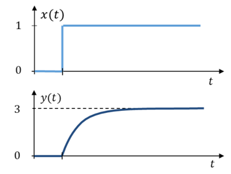
PT1 behaviour has two characteristic parameters: k_P describes the gain; τ describes the time curve of the output quantity between the step time and the steady state.

Looking back at I behaviour in the control loop

Now let us look at the control loop from the last chapter, in which A shows I behaviour.

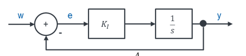
Control loop with I element (k_I and 1/s)

\[ \begin{gathered} H_{\mathrm{FÜ}} = \frac{A}{1 + A} \\[6pt] A = k_I \cdot \frac{1}{s} \\[6pt] H_{\mathrm{FÜ}} = \frac{k_I \cdot \frac{1}{s}}{1 + k_I \cdot \frac{1}{s}} = \frac{1}{1 + \frac{1}{k_I} \cdot s} \\[6pt] \text{General PT1 behaviour: } H_{\mathrm{PT1}}(s) = \frac{k_P}{1 + \tau \cdot s} \end{gathered} \]

The transfer function of the reference response is very similar to general PT1 behaviour. We determine the characteristic parameters by comparing coefficients. To do this, the two formulas are set equal.

\[ \begin{gathered} \text{General formula for PT1 behaviour: } H_{\mathrm{PT1}} = \frac{k_P}{1 + \tau \cdot s} \\[6pt] A \text{ with I behaviour in the control loop: } H_{\mathrm{FÜ}} = \frac{1}{1 + \frac{1}{k_I} \cdot s} \\[6pt] \text{Set equal: } H_{\mathrm{PT1}} = H_{\mathrm{FÜ}} \rightarrow \frac{k_P}{1 + \tau \cdot s} = \frac{1}{1 + \frac{1}{k_I} \cdot s} \\[6pt] \text{Determining the characteristic parameters by comparing coefficients:} \\[6pt] k_{P,\mathrm{FÜ}} = 1 \text{ and } \tau_{\mathrm{FÜ}} = \frac{1}{k_I} \\[6pt] H_{\mathrm{FÜ}}(s) = \frac{k_{P,\mathrm{FÜ}}}{1 + \tau_{\mathrm{FÜ}} \cdot s} \end{gathered} \]

With the parameter k_I we can set τ_FÜ. The larger k_I, the smaller τ_FÜ. The smaller τ_FÜ, the faster the output of the system reaches its final value. Let us look at the step response of the controlled system:

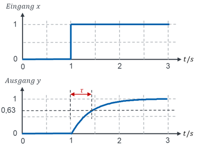
Step at input x at t = 1 s and PT1 step response y with time constant τ — Eingang = input · Ausgang = output

\[ \begin{gathered} k_{P,\mathrm{FÜ}} = 1 \\[6pt] \text{Read off: } \tau_{\mathrm{FÜ}} = \frac{1}{k_I} = 0.8\,\mathrm{s} \rightarrow k_I = 1.25 \end{gathered} \]

When does the output value reach its final value? Theoretically it never reaches it completely. In practice it reaches 99 % of the final value after the time t = 5τ. After the time t = 5τ we assume that the output quantity has settled at its final value.

Wikipedia