Control Engineering › System Behaviors 1

I Behavior

I behaviour describes integrating behaviour. A system shows I behaviour if its output quantity corresponds to the integral of the input quantity over time. Storage elements integrate their inflow, which is why storage elements show I behaviour.

Storage elements can be described well with the water model. Water storage is described by the parameters inflow, outflow and fill level. The simplest storage element is a bucket filled with water. For possible uses and the mathematics used to describe them, see the chapter Storage. Storage elements show the following relationship between input and output:

\[ \begin{gathered} y\text{: output} \\[6pt] x\text{: input} \\[6pt] y(t) = k_I \cdot \int x(t)\,dt + y_0 \end{gathered} \]

The transfer function H is not constant over time, because the time t appears in the relationship between input and output. The factor k_I is considered later. Let us first simplify the behaviour by setting x(t) to a constant value. This is no longer a general solution but a strong simplification.

\[ \begin{gathered} \text{Set } x(t) = 1 \text{ and } y_0 = 0 \\[6pt] y(t) = k_I \cdot \int x(t)\,dt + y_0 = k_I \cdot \int 1\,dt + 0 = k_I \cdot t \end{gathered} \]

If a quantity is integrated over time, it is summed up. If the inflow of a storage element is constant, its fill level rises linearly. We see this above in the simplification for x(t) = 1. The result is a proportional relationship between the output quantity y(t) and the time t.

\[ \begin{gathered} \text{Straight-line equation: } y(t) = k_I \cdot t \\[6pt] \text{Slope: } m = k_I \end{gathered} \]

Step response

With a step excitation in the input signal, x(t) jumps from 0 to 1. While x(t) = 0 applies, the output y(t) remains unchanged. A storage element without inflow does not change its fill level. After the step, x(t) = 1 applies, just as in the simplification above. The following step response results:

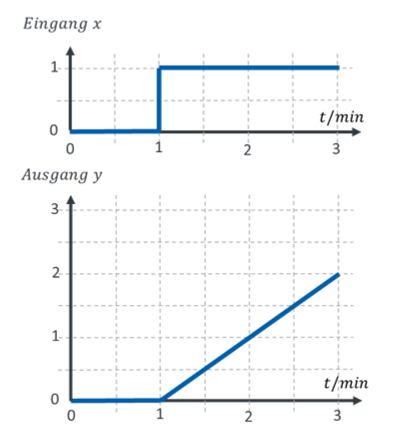
Step at input x at t = 1 min and linearly rising output y — Eingang = input · Ausgang = output

\[ \begin{gathered} y(t) = k_I \cdot \int x(t)\,dt + y_0 \\[6pt] \text{Assumption: } y_0 = 0 \\[6pt] \text{Step of } x(t) \text{ from 0 to 1 at } t = 1\,\mathrm{min} \\[6pt] \text{Slope of the line: } m = k_I \end{gathered} \]

The slope of the line is characteristic for describing I behaviour. It is generally called k_I. Concrete storage elements have different values of k_I.

We can draw two conclusions from the step response of a storage element:

1. The step response is a straight line. So it is I behaviour.

2. The slope of the line corresponds to the characteristic parameter for I behaviour: k_I.

The parameter y₀ indicates what value the output had before integration starts. It describes, for example, the fill level of a bucket before the inflow is opened. Integration then only covers the inflow. The new fill level, however, is the old fill level plus the integral of the inflow over time.

Example: car

We look at a car journey on holiday. The input quantity is the speed of the car v. The output quantity is the distance s already travelled. If a car drives at constant speed, the distance travelled keeps increasing. If the car stops, the distance already travelled is not 0; it stays unchanged. This is typical of I behaviour: when the input quantity is 0, the output quantity is not 0 (unlike P behaviour). The distance travelled depends on the speed at which you have already driven in the past. The following applies:

\[ \begin{gathered} v = \frac{ds}{dt} \text{ (school physics)} \\[6pt] \text{Integration: } s(t) = \int v(t)\,dt + s_0 \\[6pt] k_I = 1 \\[6pt] \text{with } s_0\text{: distance already travelled before} \end{gathered} \]

The value of k_I corresponds to the factor in front of the integral. In this example it is 1.

Example: bucket

For the bucket:

\[ \begin{gathered} \text{Fill level } h = \frac{1}{A} \cdot \int \dot{v}(t)\,dt + h_0 \\[6pt] k_I = \frac{1}{A} \\[6pt] \text{with } A\text{: area of the bucket, } \dot{v}(t)\text{: inflow or outflow of water} \end{gathered} \]

Example: moving mass

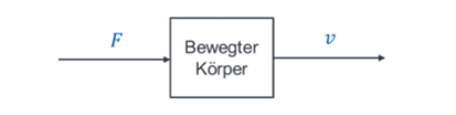
A mass is moved by a force F. I can set a football of mass m in motion with velocity v using a force F. How does such a motion behave mathematically? Moving masses show I behaviour.

A moving body continues to move at constant speed (output ≠ 0) if no external forces (input = 0) act on it. That is a sure sign of I behaviour. A space probe far away from all celestial bodies, for example, keeps flying straight ahead at almost constant speed without forces accelerating it. That bodies slow down in flight is due to external forces such as friction.

The input of such a system is a force acting on the moving body from outside. The output is its speed. The following applies:

Moving body block with input force F and output speed v — Bewegter Körper = moving body

\[ \begin{gathered} F(t) = m \cdot a(t) \rightarrow a(t) = \frac{F(t)}{m} \\[6pt] \text{from school: } a = \frac{v}{t} \rightarrow \text{in general: } a(t) = \frac{dv(t)}{dt} \\[6pt] v(t) = \int a(t)\,dt = \frac{1}{m} \int F(t)\,dt \\[6pt] k_I = \frac{1}{m} \end{gathered} \]

Example: capacitor

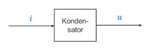
In electrical engineering, capacitors and inductors are used as storage elements. For the capacitor:

Capacitor block with input current i and output voltage u

\[ \begin{gathered} u(t) = \frac{1}{C} \int i(t)\,dt \\[6pt] k_I = \frac{1}{C} \end{gathered} \]

Systems with saturation (“Ausgleich”)

Theoretically, the output value of a storage element keeps rising as long as an input value is present. The fill level of the bucket keeps rising as long as water flows in. In practice this is of course impossible. The bucket overflows when it is full and even more water flows in. This usually applies at both limits, upper and lower. You cannot empty an empty bucket any further either.

We call the effect of overflowing “Ausgleich” (levelling off). A storage element with this effect tends towards a constant final value when completely full. Until it is completely full or empty, it shows integrating behaviour. (Strictly speaking, this is a limitation or saturation. In the technical literature, a “self-regulating plant” (German: Strecke mit Ausgleich) usually means a system that reaches a new constant final value by itself after a step, e.g. with PT1 behaviour. A pure I plant is called “non-self-regulating” (Strecke ohne Ausgleich) there.)

Let us look at the step response of an example system with I behaviour and saturation at the value 1.5:

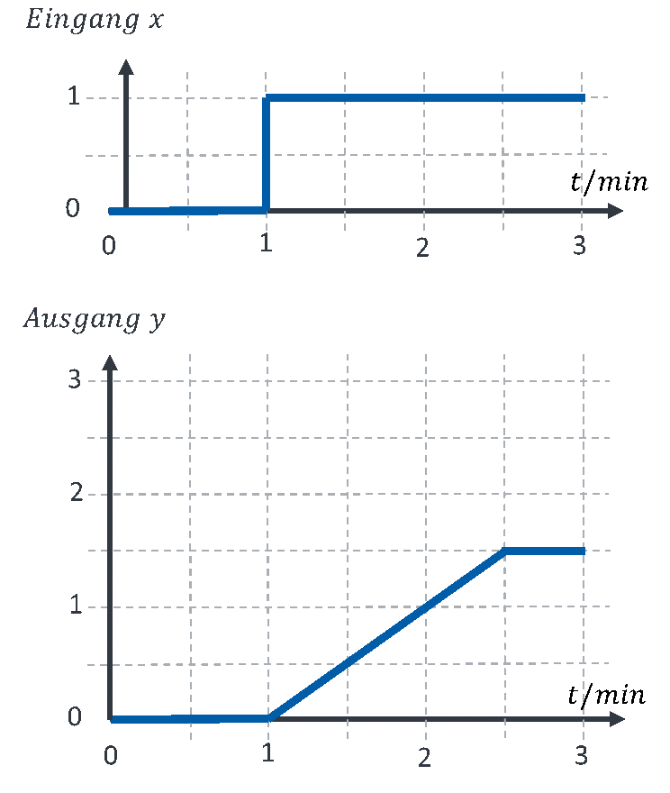
Step at input x and output y that rises linearly and remains constant from t = 2.5 min — Eingang = input · Ausgang = output

You should always operate a system in a range in which the saturation does not yet take effect. Otherwise you get behaviour that you had not calculated beforehand. Make sure that, figuratively speaking, the bucket never overflows or runs empty.