Control Engineering › System Behaviors 1

Laplace Transform

Just as in Fundamentals of Electrical Engineering, in control engineering we also use the Laplace transform to describe function blocks mathematically more simply. In I behaviour in the last chapter, an integration already appeared. Further behaviours do not make the mathematics any prettier. The Laplace transform offers the following helpful advantages:

1. An integration in the time domain becomes a product with 1/s in the frequency domain (for purely sinusoidal quantities, with 1/jω).

2. A derivative in the time domain becomes a product with s in the frequency domain (for purely sinusoidal quantities, with jω).

Complex frequency

Control engineers use a slightly different frequency parameter from electrical engineers. The angular frequency ω from electrical engineering is extended. The complex frequency is generally defined as follows:

\[ \begin{gathered} s = \sigma + j\omega \\[6pt] \omega\text{: angular frequency from electrical engineering} \\[6pt] \sigma\text{: damping of a sinusoidal waveform} \end{gathered} \]

In electrical engineering, we have so far only considered permanent sinusoidal oscillations. Permanent undamped oscillations, whose peak value does not change over time, are always calculated with s = jω, i.e. σ = 0. That is why the lazy electrical engineers only use the part s = jω in AC calculations. The parameter σ defines the damping of a sinusoidal oscillation. If, for example, the peak value of a sinusoidal oscillation keeps decreasing over time, a σ is involved.

Consider, for example, the oscillation of a swing that you let go of. The swing moves back and forth with the angular frequency ω. But it also slows down and at some point stops. The reasons are friction and air resistance. Braking leads to damping of the oscillation. For σ < 0 an oscillation is damped. For σ = 0 it is undamped and does not change over time. For σ > 0 the oscillation is even amplified; its amplitude keeps increasing. This happens if you push the swing regularly at the right moment. But we do not consider that further here.

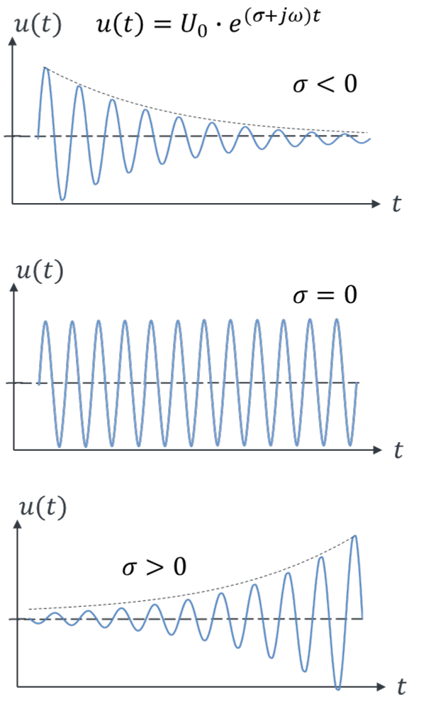
Curve of u(t) = U0 · e^((σ+jω)t) for σ < 0 (decaying), σ = 0 (constant amplitude) and σ > 0 (growing)

In this tutorial we only consider damped systems later, so you can ignore σ for now. In control engineering we use the complex frequency s wherever we use jω in electrical engineering. That is tradition, and you will be confronted with it in everyday working life. That is why I introduce s now. Mathematically, we always replace jω by s in the equations.

At first glance, the description with s is much simpler than the one with jω, because complex numbers no longer appear in the calculations. But the complex numbers are only hidden, because of course s is complex. In control engineering, however, the calculations look quasi-real, and the complex numbers remain “encapsulated” in s.

\[ \begin{gathered} \text{Time domain: } y(t) = k_I \int x(t)\,dt + y_0 \text{ with } y_0 = 0 \\[6pt] \text{Frequency domain, electrical engineering: } y(\omega) = \frac{1}{j\omega} \cdot k_I \cdot x(\omega) \\[6pt] \text{Frequency domain, control engineering: } y(s) = \frac{1}{s} \cdot k_I \cdot x(s) \\[6pt] H(s) = \frac{\text{output}}{\text{input}} = \frac{y(s)}{x(s)} = \frac{1}{s} \cdot k_I \end{gathered} \]

I behaviour as a time function is described by an integral equation. It is mathematically much simpler if we calculate with s in the frequency domain. I behaviour is then only a multiplication by the factor k_I / s.

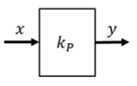
We usually split the factors of the integration into two blocks. The factor k_I on its own shows P behaviour. The factor 1/s indicates that I behaviour is present here.

\[ \text{General modelling of I behaviour in the frequency domain} \]

Blocks k_I and 1/s in series from x to y

P behaviour can also be represented in the frequency domain with a complex transfer function. Fortunately, it is exactly the same as in the time domain, because for P behaviour:

\[ \begin{gathered} y(t) = k_P \cdot x(t) \\[6pt] y(s) = k_P \cdot x(s) \\[6pt] H(s) = k_P \end{gathered} \]

Important addition: the letter “s” is already used for seconds. When real systems are controlled, both seconds and s as the complex frequency appear in the formulas. To avoid confusion, the second is always shown in bold as s in such cases; the complex frequency s is not.

Video on the purpose of transforms (German)