Measurement Technology › Offset in Signals

Differential Amplifier

The differential amplifier is an op-amp circuit with two input voltages and one output voltage. It has the following circuit diagram:

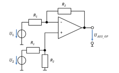
\[ U_{\mathrm{Aus,OP}} = \frac{R_2}{R_1} \cdot (U_2 - U_1) = v \cdot (U_2 - U_1) \text{ with } v = \frac{R_2}{R_1} \]

This circuit forms the difference between two input voltages. The voltage at the “+” input has the positive sign. The voltage at the “−” input has the negative sign. So it does matter which voltage we connect to which input. The voltages are not connected directly to the op-amp inputs, but again via a resistor network.

The formula for the output voltage can be interpreted as the product of a positive gain v and the voltage difference. The two identically named pairs of resistors again each have the same value.

I derived the formula for the output voltage for the summing amplifier. You can try deriving the output voltage of the differential amplifier yourself using the same approach. The solution is already given for checking.

Hint: you determine the voltage U_R2 using the voltage divider of U₂, R₁ and R₂. Let the mesh with the source U₁ run via U_R2.

Let us look again at a sensor voltage with an offset. The differential amplifier is excellent for eliminating the offset. Again we use a shift voltage, which we use either for U₁ or for U₂. In one case it acts positively and in the other negatively on the sensor signal.

The gain of the differential amplifier is positive. That of the summing amplifier is negative. With the differential amplifier, the signal is therefore shifted completely into the positive voltage range by the operation U₂ − U₁, so that the lower limit is 0 V. Then it is multiplied by a positive gain.

Let us look again at the example of the PT100 on the current source.

\[ \begin{gathered} R_{\mathrm{PT100}} = 100\,\Omega + 0.4\,\frac{\Omega}{°\mathrm{C}} \cdot T \text{ with } I_0 = 10\,\mathrm{mA} \rightarrow U_S = [1\,\mathrm{V} \ldots 1.4\,\mathrm{V}] \\[6pt] \text{ADC: } U_{\mathrm{Ref}} = 3\,\mathrm{V} \rightarrow U_{\mathrm{Ein,ADC}} = [0\,\mathrm{V} \ldots 3\,\mathrm{V}] \\[6pt] \text{Set } U_2 = U_S \text{ and } U_1 = U_V = 1\,\mathrm{V} \\[6pt] U_S - U_V = U_2 - U_1 = [1\,\mathrm{V} \ldots 1.4\,\mathrm{V}] - 1\,\mathrm{V} = [0\,\mathrm{V} \ldots 0.4\,\mathrm{V}] \end{gathered} \]

Sensor voltage U_S between 1 V and 1.4 V and difference U_S − U_V between 0 V and 0.4 V

\[ \begin{gathered} U_{\mathrm{Aus,OP}} = v \cdot (U_2 - U_1) \rightarrow v = \frac{U_{\mathrm{Ref}}}{(U_2 - U_1)_{\mathrm{max}}} = \frac{3\,\mathrm{V}}{0.4\,\mathrm{V}} = 7.5 \\[6pt] v = \frac{R_2}{R_1} \rightarrow \text{e.g. } R_1 = 1\,\mathrm{k\Omega} \text{ and } R_2 = 7.5\,\mathrm{k\Omega} \end{gathered} \]

Simulation

Output voltage U_Aus,OP rises from 0 V at 0 °C to 3 V at 100 °C

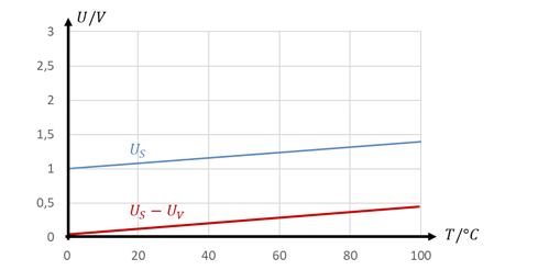
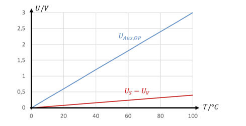
The sensor corresponds to the source U₂. The shift voltage corresponds to the source U₁. In this way, we can work with a positive shift voltage that is subtracted from the sensor voltage. The advantage of the solution with the differential amplifier is that no negative shift voltage is needed, which is difficult to provide in practice.

Superposition theorem

Note: this digression is not relevant for the exam. It deals with the following questions:

1. How do you actually calculate the output voltage of a circuit with several input voltages?

2. Why must the differential amplifier have a voltage divider at the non-inverting input (at source U₂)?

To answer both questions, we look at a fake differential amplifier without a voltage divider at the non-inverting input (at source U₂). Both questions are easier to answer with this circuit. Note: this circuit is not useful in practice; it is only used here for explanation.

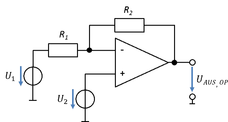
Simplified differential amplifier: U_1 via R_1 at the minus input, U_2 directly at the plus input

To calculate circuits with two input sources, the superposition theorem is applied. It works as follows: first, the first source is set to U₁ = 0 V. We calculate how the output voltage behaves as a function of the other source U₂. With U₁ = 0 V, we have a non-inverting amplifier. Because U₁ = 0 V, the source U₁ can be replaced by a short circuit. The following applies:

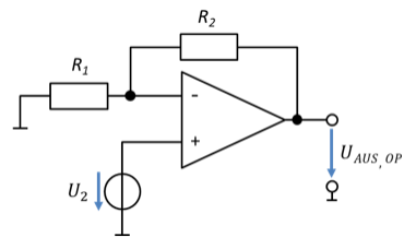
Superposition part 1: only U_2 acts, U_1 is short-circuited (non-inverting amplifier)

\[ U_{\mathrm{Aus,OP\ Teil\ 1}} = \left(1 + \frac{R_2}{R_1}\right) \cdot U_2 \]

Then the second source is set to U₂ = 0 V. We calculate how the output voltage behaves as a function of the other source U₁. With U₂ = 0 V, we have an inverting amplifier. The source U₂ can be replaced by a short circuit. The following applies:

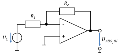
Superposition part 2: only U_1 acts, plus input at ground (inverting amplifier) — Aus = out (output)

\[ U_{\mathrm{Aus,OP\ Teil\ 2}} = -\frac{R_2}{R_1} \cdot U_1 \]

Then the sum of the two partial output voltages is formed. The following applies (Teil = part):

\[ \begin{gathered} U_{\mathrm{Aus,OP}} = U_{\mathrm{Aus,OP\ Teil\ 1}} + U_{\mathrm{Aus,OP\ Teil\ 2}} \\[6pt] U_{\mathrm{Aus,OP}} = \left(1 + \frac{R_2}{R_1}\right) \cdot U_2 - \frac{R_2}{R_1} \cdot U_1 \\[6pt] U_{\mathrm{Aus,OP}} = U_2 + \frac{R_2}{R_1} \cdot U_2 - \frac{R_2}{R_1} \cdot U_1 \\[6pt] U_{\mathrm{Aus,OP}} = U_2 + \frac{R_2}{R_1} \cdot (U_2 - U_1) \end{gathered} \]

This circuit forms the difference between the two input voltages multiplied by a gain factor. Unfortunately, the formula still contains one voltage U₂ too many. The voltage divider at the non-inverting input of the “real” differential amplifier eliminates this term from the equation. Let us look again at the circuit of the “real” differential amplifier. From the calculations above it follows:

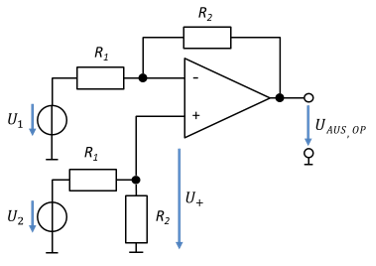
Differential amplifier with voltage divider at the plus input and voltage U_+

\[ U_{\mathrm{Aus,OP}} = \left(1 + \frac{R_2}{R_1}\right) \cdot \boldsymbol{U_+} - \frac{R_2}{R_1} \cdot U_1 \]

The voltage at the “+” input, U₊, is amplified with the formula of the non-inverting amplifier, just as in the previous circuit. Only the source U₂ is no longer applied there directly. Between U₊ and U₂, our predecessors cleverly inserted a voltage divider with:

\[ U_+ = \left(\frac{R_2}{R_1 + R_2}\right) \cdot U_2 \]

So at the output of the op-amp, the following applies:

\[ \begin{gathered} U_{\mathrm{Aus,OP}} = \left(1 + \frac{R_2}{R_1}\right) \cdot U_+ - \frac{R_2}{R_1} \cdot U_1 \\[6pt] U_{\mathrm{Aus,OP}} = \left(\frac{R_1}{R_1} + \frac{R_2}{R_1}\right) \cdot U_+ - \frac{R_2}{R_1} \cdot U_1 \\[6pt] U_{\mathrm{Aus,OP}} = \left(\frac{R_1 + R_2}{R_1}\right) \cdot U_+ - \frac{R_2}{R_1} \cdot U_1 \\[6pt] \text{with } U_+ = \left(\frac{R_2}{R_1 + R_2}\right) \cdot U_2 \\[6pt] U_{\mathrm{Aus,OP}} = \left(\frac{R_1 + R_2}{R_1}\right) \cdot \left(\frac{R_2}{R_1 + R_2}\right) \cdot U_2 - \frac{R_2}{R_1} \cdot U_1 \\[6pt] \text{cancel } (R_1 + R_2) \text{ in the left term} \\[6pt] U_{\mathrm{Aus,OP}} = \frac{R_2}{R_1} \cdot U_2 - \frac{R_2}{R_1} \cdot U_1 = \frac{R_2}{R_1}(U_2 - U_1) \end{gathered} \]

We now have a formula in which the input voltages are subtracted from each other and amplified by a common factor. In my eyes, this solution is simple and elegant, and therefore brilliant.