Electrical Engineering ETR › Complex AC Analysis

Frequency Domain

In a transformation, the mathematical description and often also the way of looking at the signal are changed. The Laplace transform switches from the time domain, in which the signals are plotted over time t as the x-axis, to the frequency domain. Here, the frequency f is plotted on the x-axis. The axis begins at the zero point at f = 0 Hz, which corresponds to direct current. Negative frequencies are not meaningful in electrical engineering for now. To the right, towards high frequencies, the axis is unlimited. The higher the frequency f, the further to the right the x-value of the frequency lies in the figure.

You know some frequencies from everyday life. The mains frequency of the socket voltage in Europe is f = 50 Hz. The frequency of WLAN or Bluetooth is 2.4 GHz. You receive FM radio in the range [87.5 MHz … 108 MHz]. When the frequency f is plotted on the x-axis, we regard the frequency as a variable parameter. If the frequency of a signal does not change, that is convenient, because we then only look at one point and no longer at a continuous curve as with time.

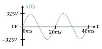
In the time domain, a signal is shown with the time t on the x-axis. The instantaneous value is shown on the y-axis. The instantaneous value is the current value that the quantity has at a point in time t. From a time curve, we can read off which instantaneous value (y-value) is present at which point in time (x-value). Here, as an example, is the voltage at the mains socket:

Time curve of the mains voltage u(t) with a peak value of 325 V over 40 ms

\[ \begin{gathered} \text{Time } t = 5\,\mathrm{ms}: u(t) = 325\,\mathrm{V} \\[4pt] \text{Time } t = 20\,\mathrm{ms}: u(t) = 0\,\mathrm{V} \end{gathered} \]

In the frequency domain, the frequency f or the angular frequency ω is plotted on the x-axis. There are two y-values: the peak value and the phase. That is why two graphs are drawn to represent a signal in the frequency domain. Here is an example for the voltage at the mains socket, plotted over the frequency f:

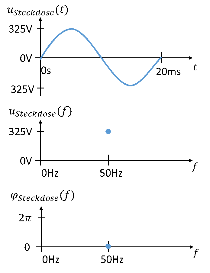
Mains voltage in the time domain and in the frequency domain: peak value 325 V and phase 0 at 50 Hz — Steckdose = socket outlet

The top of the figure shows the voltage curve in the time domain. The bottom shows the two graphs of the frequency domain. Peak value and phase each result in only one point, because the frequency at the mains socket does not change. In the “frequency domain”, the voltage at the mains socket consists only of a peak value and an associated phase. In later lectures, you will also get to know voltages composed of several parts. If the voltages have different frequencies, there are also several points in the frequency domain. Let us look at an example of this as well:

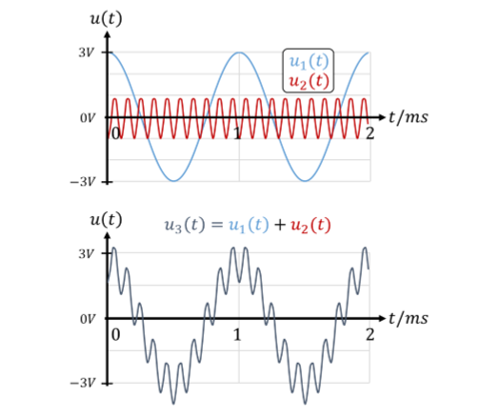
\[ \begin{gathered} u_1(t) = 3\,\mathrm{V} \cdot \sin\left(\omega t + \frac{\pi}{2}\right) \text{ with } f = 1\,\mathrm{kHz} \rightarrow T = 1\,\mathrm{ms} \\[4pt] u_2(t) = 1\,\mathrm{V} \cdot \sin\left(\omega t - \frac{\pi}{2}\right) \text{ with } f = 10\,\mathrm{kHz} \rightarrow T = 0.1\,\mathrm{ms} \\[4pt] u_3(t) = u_1(t) + u_2(t) \end{gathered} \]

Time curves of u1(t) at 1 kHz, u2(t) at 10 kHz and the sum u3(t)

In the figure above, we see two time curves of voltages. In the light-blue voltage u₁(t), the period is T = 1 ms. This corresponds to the frequency f = 1 kHz. In the red voltage u₂(t), the period is T = 0.1 ms. This corresponds to the frequency f = 10 kHz. We can simply read off the peak values on the y-axis.

The dark-blue voltage u₃(t) contains two frequencies. After all, the voltage consists of two partial voltages (light blue and red) with different frequencies. This voltage is difficult to analyse in the time domain. Or can you recognise the parameters of the light-blue and the red voltage from the time curve of the dark-blue voltage? That is why we prefer to show this sum voltage in the frequency domain:

Peak values and phases of u1 (1 kHz) and u2 (10 kHz) in the frequency domain

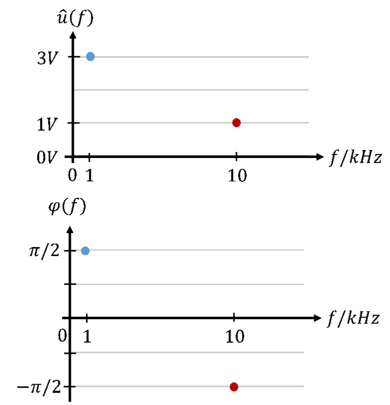
The upper diagram shows the peak values of the two voltages over the frequency f as the x-axis. The lower diagram shows the phases of both voltages. In the frequency domain, each voltage is assigned a peak value and a phase. In the frequency domain, each voltage component in a sum voltage gets its own point for peak value and phase. In this representation, it is very easy to read off the parameters of a sum voltage directly.