Unwanted Filters

The entire chapter “Unwanted filters” is not relevant for the exam. You can leave it out if you only want to prepare quickly for the lecture.

Let us look at movements in everyday life. You can throw a ball up and catch it once a minute. You can also manage that ten times a minute. If you are supposed to do it once a second, it already gets tight. The faster you throw and catch the ball, the less high you can throw it. So the peak value “throw height” decreases with frequency. In your ability to throw a ball up and catch it, you are low-pass limited.

Every system is low-pass limited in everything at some point. Nothing happens infinitely fast. You do not need to actively filter anything for this; it happens all by itself. A filter deliberately added to a system supplements this natural behaviour of systems.

All real circuits and components show natural low-pass behaviour in their function. The signals at the output of a system cannot change arbitrarily fast. We look at the phenomenon using the example of operational amplifiers. Let us take an op-amp that amplifies an AC input signal by a factor of v = −1000.

According to the data sheet, the op-amp has a maximum rate of change of its output voltage: the slew rate (maximum voltage slope). An op-amp with a slew rate of 1 V/µs cannot change its voltage by more than 1 V if we give it one microsecond. A signal with a frequency of f = 1 MHz moves up and down once completely within one microsecond. Let us use f = 1 MHz as the signal frequency for the example and look at the output signal of the op-amp:

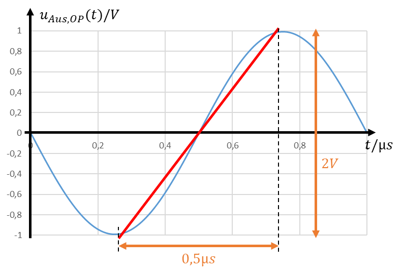
The output signal of the op-amp changes by 2 V between the times 0.25 µs and 0.75 µs. Let us pretend that the change is linear (red curve). Then the op-amp would have to change its output voltage by 2 V within 0.5 µs, i.e. at 4 V/µs. It cannot manage that; its output is not fast enough.

In the water model analogy, the op-amp has a pipe with a limited diameter at its output. Only a limited amount of water per unit time fits through this pipe, so the water level at the output of the op-amp cannot change arbitrarily fast.

The op-amp cannot generate this output signal. So it generates the largest signal it can still manage:

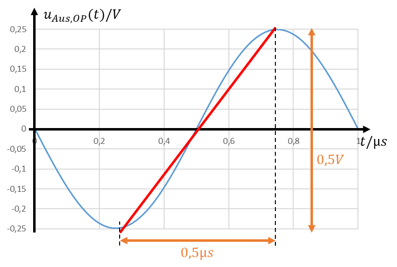
Let us look at an op-amp output voltage with a peak value of 0.25 V. If the voltage rise between the extreme values of the output voltage were linear, the op-amp output would have to rise by 0.5 V in 0.5 µs. It can manage that, because it can change its output by 1 V/µs. (With an exactly sinusoidal waveform, the maximum slope is 2πf ∙ û. Then at 1 MHz the op-amp only manages a peak value of about 0.16 V.)

The higher the frequency of the input voltage, the steeper the voltage rise for the same peak value. There is less time for the same voltage rise when the period becomes shorter because the frequency increases. Let us look at an op-amp output voltage at a 10 times higher frequency. The op-amp can then only deliver 1/10 of the output voltage. So the output voltage of the op-amp shows low-pass behaviour without anyone having connected an R or C externally.

Gain-bandwidth product

There are further influencing factors within an op-amp that determine its low-pass behaviour. All these effects are subject to scatter or uncertainty as to when they take effect. So an op-amp initially has low-pass behaviour with a cut-off frequency that is determined by many effects and therefore has an uncertain value. That is rubbish. Internally, therefore, a dominant low-pass filter is created with a resistor and a capacitor, whose cut-off frequency is set by the manufacturer. In the Bode plot, the low-pass cut-off frequency of this deliberately added filter lies further to the left than all other natural cut-off frequencies. This ensures deterministic and always identical behaviour of all op-amps in a series.

If the op-amp can no longer provide a desired output voltage, its gain effectively decreases. The gain of the op-amp corresponds to its transfer function H. As with all other filters, the transfer function thus shows low-pass behaviour. This can look like this:

This example op-amp can amplify DC signals with a maximum gain of |v| = 100000. The higher the signal frequency at the input, the lower the gain. Input signals with f = 1 MHz are only amplified with |v| = 1. The frequency range up to which a desired gain can still be achieved is called the “bandwidth”. So this op-amp has a bandwidth of 1 MHz if we need, for example, v = −1. If this op-amp is to amplify an input signal with v = −1000, this only works up to a signal frequency of 1 kHz.

The “gain-bandwidth product” of an op-amp is a constant given in the data sheet. For the example op-amp it is 1 MHz. The product of gain and bandwidth is always 1 MHz for every point on the red line to the right of the cut-off frequency.

The op-amp can serve any operating point below the red curve. The red line only limits its gain from above. For example, the op-amp can also be operated at f = 1 kHz with a gain of v = 10.

This low-pass behaviour has nothing directly to do with the slew rate from above. With the low-pass behaviour from the Bode plot, the op-amp is artificially slowed down so that its behaviour is deterministic. For this, the cut-off frequency of the low-pass behaviour must lie so far to the left in the Bode plot that all other effects do not come into play in the first place.

It is as if the low-pass filter made the ball move so slowly that you can always catch and throw it easily. The ball then flies, for example, at a maximum frequency of f = 0.1 Hz. Nobody then notices that you can only catch and throw the ball up to a frequency of f = 1 Hz. By deliberately slowing down, you pre-empt the natural cut-off frequency so that it no longer has any effect externally.