Measurement Technology › Filters Part 2 › Filter Types

Band-Pass Filter

A band-pass filter combines high-pass and low-pass behaviour. In the range around the useful frequency it amplifies with |H(ω)| = 1. The band-pass filter has two cut-off frequencies. The lower cut-off frequency is that of the high-pass filter, the upper one that of the low-pass filter. A band-pass filter is used when interference with both high and low frequencies is contained in the useful signal.

Let us look at the following example (Nutz = useful, Stör = interference):

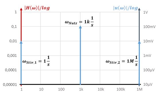
Spectrum: interference signal at 1 1/s, useful signal at 1k 1/s, interference signal at 1M 1/s — Nutz = useful · Stör = disturbance

\[ \begin{gathered} u_{\mathrm{Sensor}} = u_{\mathrm{Nutz}} + u_{\mathrm{Stör},1} + u_{\mathrm{Stör},2} \\[6pt] u_{\mathrm{Nutz}}(t) = 100\,\mathrm{mV} \cdot \sin(\omega_{\mathrm{Nutz}} t);\ \hat{u}_{\mathrm{Nutz}} = 100\,\mathrm{mV};\ \omega_{\mathrm{Nutz}} = 1\mathrm{k}\,\tfrac{1}{\mathrm{s}} \\[6pt] u_{\mathrm{Stör},1}(t) = 10\,\mathrm{mV} \cdot \sin(\omega_{\mathrm{Stör},1} t);\ \hat{u}_{\mathrm{Stör},1} = 10\,\mathrm{mV};\ \omega_{\mathrm{Stör},1} = 1\,\tfrac{1}{\mathrm{s}} \\[6pt] u_{\mathrm{Stör},2}(t) = 10\,\mathrm{mV} \cdot \sin(\omega_{\mathrm{Stör},2} t);\ \hat{u}_{\mathrm{Stör},2} = 10\,\mathrm{mV};\ \omega_{\mathrm{Stör},2} = 1\mathrm{M}\,\tfrac{1}{\mathrm{s}} \end{gathered} \]

Both interference signals should be attenuated as much as possible by the filter. Around the useful signal, the filter should let the signal pass unchanged with |H| = 1. The further we move the filter’s cut-off frequencies away from the interference frequencies, the better the filter attenuates the interference signals.

For attenuation, it would be advantageous to place the cut-off frequencies as close as possible to the useful frequency. So that the useful signal remains unaffected by the filters, we again keep a minimum distance of a factor of 10 between the useful frequency and the filter frequencies. So we place a range with |H| = 1 between 100 1/s and 10k 1/s. To the right of this range the low-pass filter should act, to the left of it the high-pass filter. The behaviour of the desired filter is shown in the following figure (HP = high-pass, TP = low-pass):

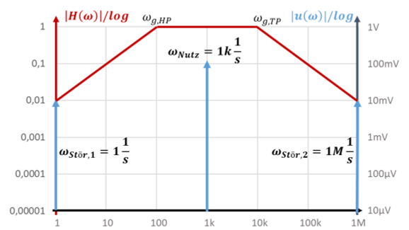
Desired band-pass filter: rise up to ω_g,HP, pass band up to ω_g,TP, then fall — Nutz = useful · Stör = disturbance

\[ \begin{gathered} \omega_{g,\mathrm{HP}} = 0.1 \cdot \omega_{\mathrm{Nutz}} = 100\,\frac{1}{\mathrm{s}} \\[6pt] \omega_{g,\mathrm{TP}} = 10 \cdot \omega_{\mathrm{Nutz}} = 10\mathrm{k}\,\frac{1}{\mathrm{s}} \end{gathered} \]

The high-pass filter and the low-pass filter each act on all frequencies. The high-pass filter only attenuates signals with frequencies to the left of the high-pass cut-off frequency ω_g,HP = 100 1/s. Signals to the right of this cut-off frequency all pass the filter unchanged with |H| = 1. The signals to the right of the low-pass cut-off frequency ω_g,TP = 10k 1/s are attenuated by the low-pass filter. However, the low-pass filter lets all signals with frequencies to the left of this cut-off frequency pass unchanged. So the filters do not influence each other.

Implementation

Filters can be connected in series. A high-pass filter and a low-pass filter can be combined into a band-pass filter. Whenever two circuit sections are connected, a matching problem arises. Matching can be achieved by connecting a passive filter to the output of the operational amplifier of an active filter. As an example, I show an active low-pass filter followed by a passive high-pass filter. The transfer functions of the sub-circuits are already known.

Active low-pass filter followed by a passive RC high-pass filter made of C_3 and R_3 — Aus = out (output) · Ein = in (input)

\[ \begin{gathered} |H_{\mathrm{OP}}(\omega)| = \left|\frac{u_{\mathrm{Aus,OP}}}{u_{\mathrm{Ein}}}\right| = \left|-\frac{R_2}{R_1}\right| \cdot \left(\frac{1}{\sqrt{1 + \omega^2/\omega_{g,\mathrm{TP}}^2}}\right) \text{ with } \omega_{g,\mathrm{TP}} = \frac{1}{R_2 C_2} \\[6pt] |H_{\mathrm{Hochpass}}| = \left|\frac{u_{\mathrm{Aus}}}{u_{\mathrm{Aus,OP}}}\right| = \frac{\omega/\omega_{g,\mathrm{HP}}}{\sqrt{1 + \omega^2/\omega_{g,\mathrm{HP}}^2}} \text{ with } \omega_{g,\mathrm{HP}} = \frac{1}{R_3 C_3} \\[6pt] |H_{\mathrm{Schaltung}}| = |H_{\mathrm{OP}}| \cdot |H_{\mathrm{Hochpass}}| = \underbrace{\left|-\frac{R_2}{R_1}\right|}_{v} \cdot \underbrace{\left(\frac{1}{\sqrt{1 + \omega^2/\omega_{g,\mathrm{TP}}^2}}\right)}_{\text{low-pass}} \cdot \underbrace{\left(\frac{\omega/\omega_{g,\mathrm{HP}}}{\sqrt{1 + \omega^2/\omega_{g,\mathrm{HP}}^2}}\right)}_{\text{high-pass}} \end{gathered} \]

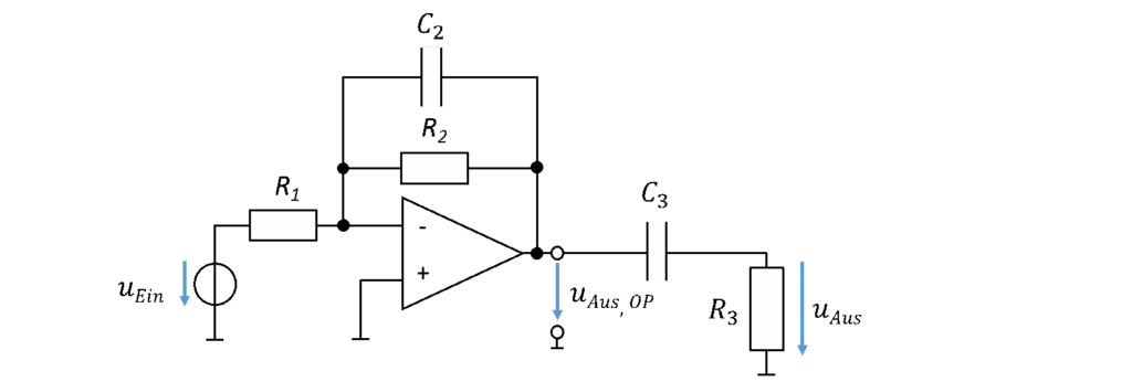
(Hochpass = high-pass, Schaltung = circuit.) The signal first passes through the active low-pass filter in the left part of the circuit. There the high-frequency interference is filtered out and the signal is amplified. So in the signal u_Aus,OP, u_Stör,2 is already attenuated.

The signal then passes through the high-pass filter made of R₃ and C₃. In this part of the circuit, the low-frequency interference is filtered out.

Although we are working with an example here, the formulas already apply as a general solution. The position of the cut-off frequencies differs from problem to problem, but you only set it when dimensioning the components.

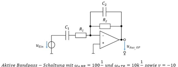
There is another circuit with which you can implement band-pass behaviour. You can build an active high-pass filter and add a passive low-pass filter at the output. You can also connect an active high-pass filter to an active low-pass filter. Combining the known circuits leaves a lot of room for creativity. Finally, I would like to show you a particularly elegant circuit:

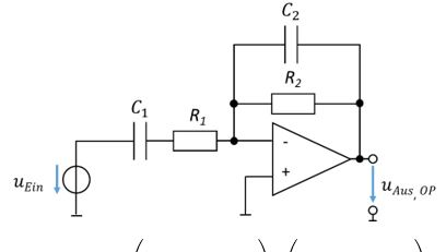
Active band-pass filter with C_1 and R_1 at the input and C_2 in parallel with R_2 — Ein = in (input)

\[ \begin{gathered} |H(\omega)| = |v| \cdot \left(\frac{1}{\sqrt{1 + \omega^2/\omega_{g,\mathrm{TP}}^2}}\right) \cdot \left(\frac{\omega/\omega_{g,\mathrm{HP}}}{\sqrt{1 + \omega^2/\omega_{g,\mathrm{HP}}^2}}\right) \\[6pt] \text{with } v = -\frac{R_2}{R_1};\ \omega_{g,\mathrm{HP}} = \frac{1}{R_1 C_1};\ \omega_{g,\mathrm{TP}} = \frac{1}{R_2 C_2} \end{gathered} \]

The high-pass filter is determined by the components R₁ and C₁. R₂ and C₂ set the low-pass cut-off frequency. I will work through an example problem with this circuit:

Example

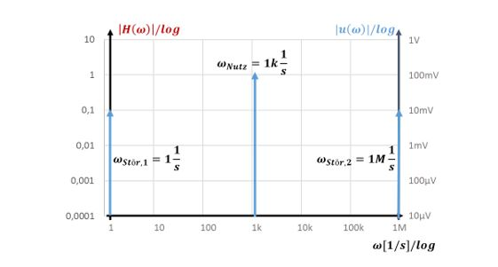
Spectrum of the task: interference signals at 1 1/s and 1M 1/s, useful signal at 1k 1/s

Goals:

Amplify the useful signal overall with \(v = -10\)
Attenuate both interference signals as much as possible

Tasks:

Draw the Bode plot for the goals
Choose a circuit and dimension the components. Set \(R_1 = 1\,\mathrm{k\Omega}\).
Calculate the signal-to-noise ratio SNR at the output of the circuit for both interferences

Solution:

\[ \begin{gathered} \text{Active band-pass circuit with } \omega_{g,\mathrm{HP}} = 100\,\tfrac{1}{\mathrm{s}} \text{ and } \omega_{g,\mathrm{TP}} = 10\mathrm{k}\,\tfrac{1}{\mathrm{s}} \text{ and } v = -10 \\[6pt] \text{Components: } R_2 = |v| \cdot R_1 = 10\,\mathrm{k\Omega};\ C_1 = \frac{1}{R_1 \omega_{g,\mathrm{HP}}} = 10\,\text{µF};\ C_2 = \frac{1}{R_2 \omega_{g,\mathrm{TP}}} = 10\,\mathrm{nF} \\[6pt] \hat{u}_{\mathrm{Nutz}} = 100\,\mathrm{mV};\ \hat{u}_{\mathrm{Stör}1} = 10\,\mathrm{mV};\ \hat{u}_{\mathrm{Stör}2} = 10\,\mathrm{mV} \\[6pt] \text{Read from the Bode plot:} \\[6pt] |H(\omega_{\mathrm{Nutz}})| = 10;\ |H(\omega_{\mathrm{Stör},1})| = 0.1;\ |H(\omega_{\mathrm{Stör},2})| = 0.1 \\[6pt] \hat{u}_{\mathrm{Aus,OP,Nutz}} = |H(\omega_{\mathrm{Nutz}})| \cdot \hat{u}_{\mathrm{Nutz}} = 10 \cdot 100\,\mathrm{mV} = 1\,\mathrm{V} \\[6pt] \hat{u}_{\mathrm{Aus,OP,Stör}1} = |H(\omega_{\mathrm{Stör}1})| \cdot \hat{u}_{\mathrm{Stör}1} = 0.1 \cdot 10\,\mathrm{mV} = 1\,\mathrm{mV} \\[6pt] \hat{u}_{\mathrm{Aus,OP,Stör}2} = |H(\omega_{\mathrm{Stör}2})| \cdot \hat{u}_{\mathrm{Stör}2} = 0.1 \cdot 10\,\mathrm{mV} = 1\,\mathrm{mV} \\[6pt] \mathrm{SSA}_{\mathrm{Störung1,Aus}} = \left|\frac{\hat{u}_{\mathrm{Aus,OP,Nutz}}}{\hat{u}_{\mathrm{Aus,OP,Stör}1}}\right| = \frac{1\,\mathrm{V}}{1\,\mathrm{mV}} = 1000 \\[6pt] \mathrm{SSA}_{\mathrm{Störung2,Aus}} = \left|\frac{\hat{u}_{\mathrm{Aus,OP,Nutz}}}{\hat{u}_{\mathrm{Aus,OP,Stör}2}}\right| = \frac{1\,\mathrm{V}}{1\,\mathrm{mV}} = 1000 \end{gathered} \]

Simulation

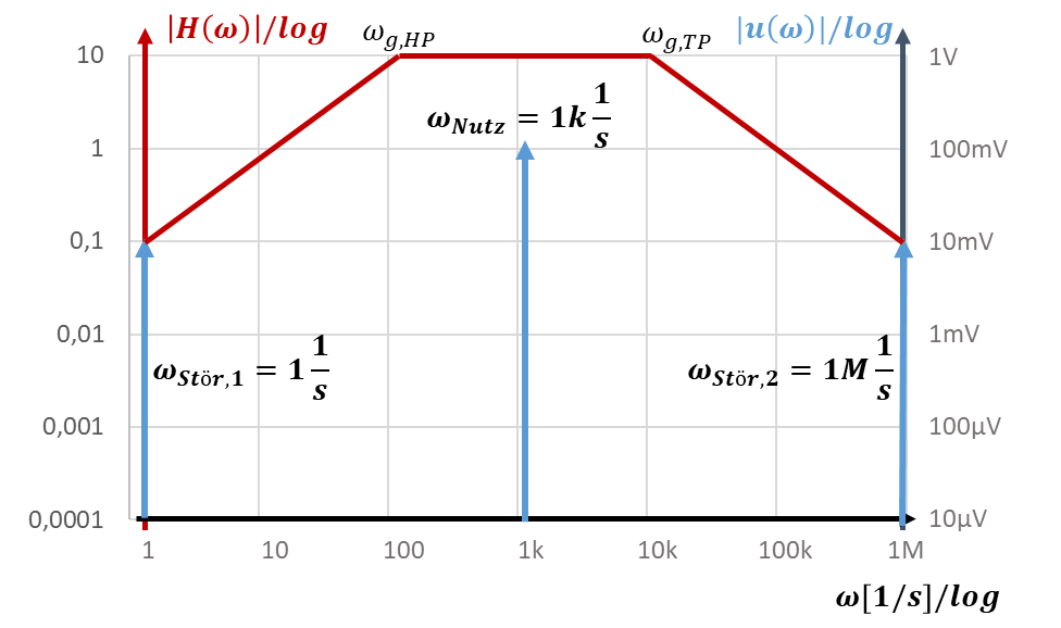
The gain v = −10 acts on all three signals. The useful signal passes all filters unchanged and is only amplified with v = −10.

The low-frequency interference signal u_Stör,1 is attenuated by a factor of 100 by the high-pass filter. This value can either be determined mathematically or read from the Bode plot. The signal passes the low-pass filter unchanged, since its frequency is so low that the low-pass filter has |H| = 1 there. Overall, the signal is amplified by a factor of −10 / 100 = −0.1.

The high-frequency interference signal u_Stör,2 is attenuated by a factor of 100 by the low-pass filter. The signal passes the high-pass filter unchanged, since its frequency is so high that the high-pass filter has |H| = 1 there. Overall, the signal is amplified by a factor of −10 / 100 = −0.1.