Control Engineering › Oscillating Systems 2

Transfer Function

In the chapter before last, we opened the control loop to determine the loop gain. Now we close the control loop again and look at the transfer function of a control loop. For this, we can insert the loop gain into the formula of the transfer function. Let us consider a system of two I blocks connected in series in a control loop. Two storage elements are involved, so an oscillation is possible. The following applies:

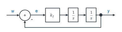
Control loop with controller k_I and two integrators 1/s

\[ \begin{gathered} A = k_I \cdot \frac{1}{s} \cdot \frac{1}{s} = \frac{k_I}{s^2} \\[6pt] \text{Loop gain: } v_R = -k_I \cdot \frac{1}{s} \cdot \frac{1}{s} = -A \\[6pt] \text{Reference response: } H_{\mathrm{FÜ}} = \frac{1}{1 + \frac{1}{A}} = \frac{1}{1 - \frac{1}{v_R}} \\[6pt] \text{Oscillation condition: } v_R = 1 \\[6pt] H_{\mathrm{FÜ}}(v_R = 1) = \frac{1}{1 - \frac{1}{v_R}} = \frac{1}{1 - 1} = \frac{1}{0} \rightarrow \infty \end{gathered} \]

When a controlled system oscillates, the denominator of its transfer function tends to 0. The transfer function itself thus becomes infinitely large. We can calculate when a system oscillates. To do this, we set the denominator of its transfer function to 0 and check whether the equation has a solution. If so, the system oscillates.

\[ \begin{gathered} H_{\mathrm{FÜ}} = \frac{1}{1 + \frac{1}{A}} = \frac{1}{1 + \frac{s^2}{k_I}} \\[6pt] \text{Set } s = j\omega \\[6pt] H_{\mathrm{FÜ}} = \frac{1}{1 - \frac{\omega^2}{k_I}} \\[6pt] \text{Oscillation when denominator} = 0 \rightarrow \frac{\omega_0^2}{k_I} = 1 \text{ or } \omega_0 = \sqrt{k_I} \\[6pt] \text{Set e.g. } k_I = 1 \rightarrow \omega_0 = 1\,\frac{1}{\mathrm{s}}\text{: “resonant angular frequency”} \\[6pt] \text{Resonant frequency } f_0 = \frac{\omega_0}{2\pi} = 0.16\,\mathrm{Hz} \\[6pt] \text{Period: } T_0 = \frac{1}{f_0} = \frac{2\pi}{\omega_0} = 6.28\,\mathrm{s} \\[6pt] \text{With } \mathrm{s}\text{: second (upright) and } s\text{: complex frequency (italic)} \end{gathered} \]

Note: here, giving times in minutes makes no sense, so seconds have been used as an exception. For seconds, the letter s is shown in bold.

There is a solution for which the denominator of the transfer function becomes 0. So the system oscillates at the angular frequency at which the denominator becomes 0. That is our resonant frequency.

The step response of an oscillating system oscillates after the input step. The time curve of the step response of the example system with k_I = 1 is shown in the figure below. The step of the input quantity in blue takes place at t = 1 s.

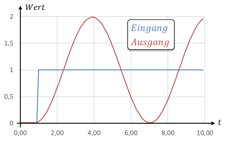
Step at the input at t = 1 and undamped oscillation of the output between 0 and 2 — Eingang = input · Ausgang = output · Wert = value

The oscillation of the output quantity starts as soon as the input steps. The period T₀ in the graph corresponds to the calculated value of T₀ = 6.28 s. It can be determined from the distance between the maxima. A sinusoidal sustained oscillation is characterised by the parameter “oscillation frequency” or “resonant frequency”. This parameter is always available as angular frequency ω, frequency f and period T.

The peak value of the oscillation is 1. After the step, the output quantity oscillates around the reference variable w = 1.

Exercise

Model the controlled system in Matlab Simulink. Excite the system with a step from 0 to 1. Vary k_I and observe how the output behaviour changes. Here is the solution for k_I = 1:

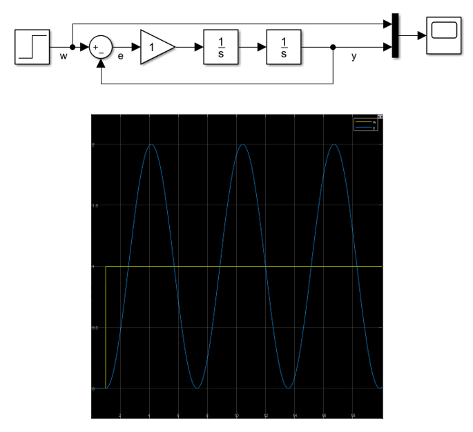
Simulation model of the control loop with step source, gain 1, two integrators and scope, and the simulated sustained oscillation

The resonant frequency depends on k_I. So we expect it to change when k_I is varied. In this control loop, the parameter k_I is like the string length of the pendulum: it influences the resonant frequency.