Electrical Engineering BMT & UFC › Charging a Storage Element

Capacitor in a Circuit

The effect of a capacitor as a store is to be illustrated with an example. You can build the corresponding circuit as an optional experiment in the lab course. The parameters of the circuit are not entirely realistic, because they are to be implemented with components available in the lab. This part of the tutorial is optional; you do not need to understand it completely for the exam.

A battery-powered circuit is to measure a temperature continuously and send the measured value once per second via a radio module to a smartphone. An app running on the smartphone displays the temperature value. For the circuit, we need a battery, an electronic thermometer and a radio module. These components are modelled first.

Modelling

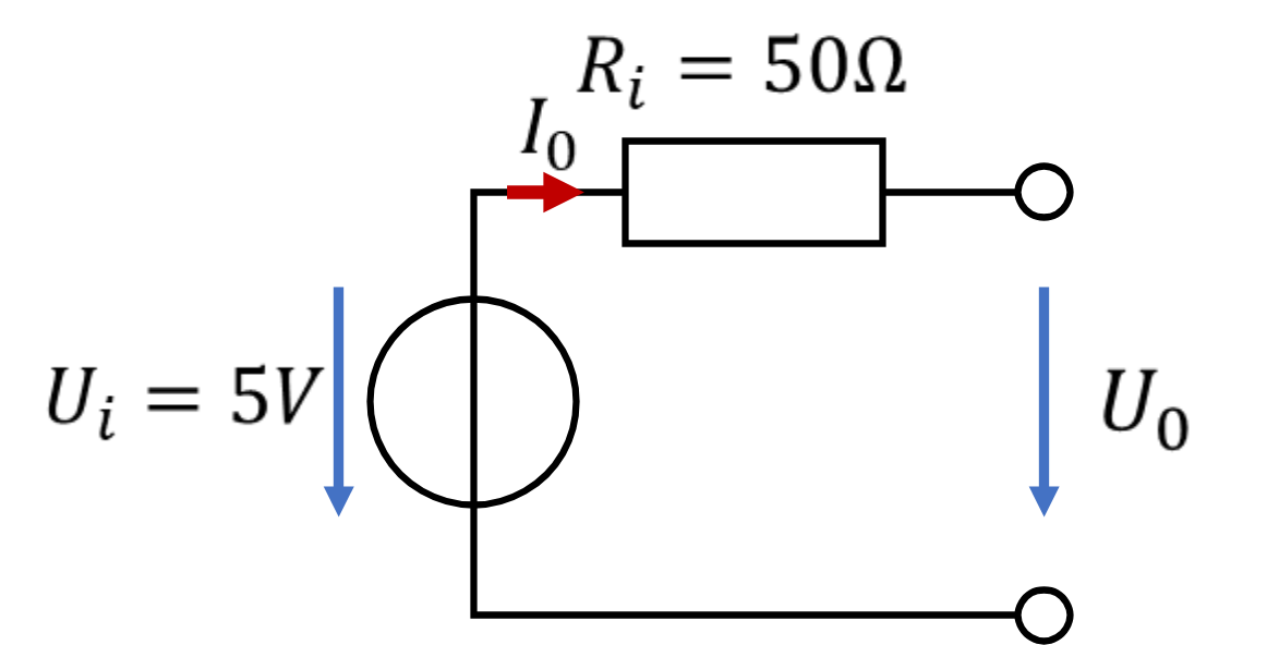
As the battery, we use a rechargeable battery as a real voltage source. It has an open-circuit voltage of U_i = 5 V and an internal resistance of R_i = 50 Ω. These are not realistic values for a rechargeable battery, but they illustrate the behaviour of a real voltage source well. The following circuit diagram shows how the battery is modelled:

Battery as a real voltage source with Ui = 5 V and Ri = 50 Ω

At an operating voltage of 5 V, the electronic thermometer needs a current of 5 mA. It is modelled as a resistor. This means that, for calculation and modelling, the relationship between voltage and current at the thermometer is calculated with Ohm's law. It is not a resistor; it has a resistance value as a property.

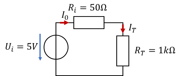
\[ R_T = \frac{5\,\mathrm{V}}{5\,\mathrm{mA}} = 1\,\mathrm{k\Omega} \]

The thermometer is connected directly to the terminals of the real battery. It is thus connected in series with the internal resistance of the battery.

For a transmission lasting 1 ms at 5 V, the radio module needs a current of 100 mA. We also model the radio module as a resistor.

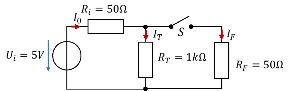
\[ R_F = \frac{5\,\mathrm{V}}{100\,\mathrm{mA}} = 50\,\Omega \]

Battery with thermometer RT and switchable radio module RF

The radio module is not permanently active; it is only switched on once per second for 1 ms. We therefore place the radio module behind a switch S. It is connected in parallel with the thermometer so that it receives the same voltage of 5 V directly from the battery. The radio module and the thermometer both need a minimum voltage of 4 V to operate.

Calculation

Whenever switch S is open, there is a voltage divider of R_i and R_T. The voltage across R_T is then:

\[ U_T = U_i \cdot \frac{R_T}{R_T + R_i} = 5\,\mathrm{V} \cdot \frac{1\,\mathrm{k\Omega}}{1\,\mathrm{k\Omega} + 50\,\Omega} = 4.76\,\mathrm{V} \]

Simulation

The voltage across the thermometer is somewhat smaller than the internal voltage of the real voltage source, because current flows out of the source. The less current flows out, the higher the output voltage of the battery.

Whenever switch S is closed, there is a parallel connection of R_T and R_F. We can calculate it as:

\[ R_{TF} = R_T \,||\, R_F = \frac{R_T \cdot R_F}{R_T + R_F} = 47.6\,\Omega \approx 50\,\Omega \]

In the parallel connection, the smaller of the resistances determines the total resistance. The voltage across the radio module is then calculated from the voltage divider

\[ U_T = U_i \cdot \frac{R_{TF}}{R_{TF} + R_i} = 5\,\mathrm{V} \cdot \frac{50\,\Omega}{50\,\Omega + 50\,\Omega} = 2.5\,\mathrm{V} \]

This voltage is far too low; neither the radio module nor the electronic thermometer can work with such a low supply voltage. The radio module draws so much current from the battery that the output voltage collapses. This happens with every real source above a certain current.

The basic current demand and the available current are plotted over time in the following graph:

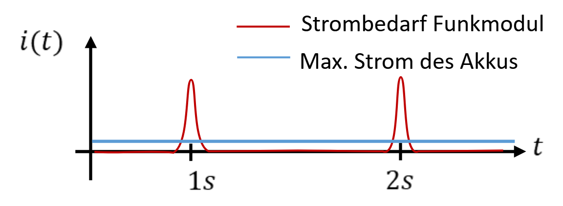
Current demand of the radio module and maximum current of the battery over time — Strombedarf = current demand · Funkmodul = radio module · Strom = current · Akkus = batteries

In this application, a capacitor helps as a charge store. The capacitor briefly provides separated charge for the radio module. It is constantly and slowly recharged. It is placed so that it is always charged and is discharged when the switch is closed. We extend the circuit as follows:

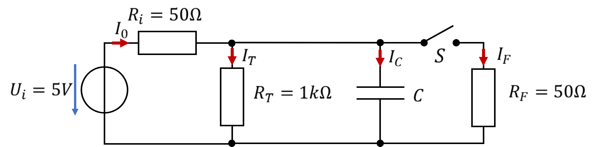
Circuit with buffer capacitor C in parallel with the radio module

Simulation

Dimensioning the capacitor

To dimension the capacitor, we look at the discharge case. With the switch open, the capacitor is charged to about 5 V (more precisely 4.76 V). We estimate the value with rounded numbers. It may be discharged to 4 V at most. So the voltage across the capacitor may drop by at most ΔU = 1 V while the radio module transmits the temperature. The current from the capacitor is I = 100 mA, flowing for the time t = 1 ms.

We pretend that the current into the radio module is constant during the time the switch is closed. This is also the time over which we integrate during the discharge process. However, this assumption only holds if the voltage across the radio module is also constant. After all, the radio module is modelled as a resistor.

So this assumption is actually not correct. We use it nonetheless, because otherwise we would have to find the antiderivative of the integral. Because we want to avoid that, we assume the current to be constant and thus deliberately make an error. At the end, we check how bad the error was. I come back to this at the very end of the chapter.

For the capacitor with constant current, the following applies:

\[ \begin{gathered} u_C(t) = U_{C0} + \frac{1}{C} \int_{0\,\mathrm{ms}}^{1\,\mathrm{ms}} i_C(t)\,dt \\[6pt] u_C(1\,\mathrm{ms}) = U_{C0} - \frac{1}{C} \cdot i_C \cdot \Delta t = U_{C0} - \Delta U \\[6pt] \Delta t = 1\,\mathrm{ms} \\[4pt] U_{C0} = 5\,\mathrm{V} \\[4pt] u_C \text{ may drop by at most } \Delta U = 1\,\mathrm{V} \\[6pt] \Delta U = \frac{i_C \cdot \Delta t}{C} = 1\,\mathrm{V} \\[6pt] C = \frac{i \cdot \Delta t}{\Delta U} = \frac{100\,\mathrm{mA} \cdot 1\,\mathrm{ms}}{1\,\mathrm{V}} = 100\,\text{µF} \end{gathered} \]

Both loads need a voltage of at least 4 V. The change in voltage across the capacitor may therefore be at most ΔU = 5 V – 4 V = 1 V. In the last line, the equation between voltage and current has been solved for the capacitance C. A capacitor with C = 100 µF should be sufficient for the voltage at the battery output to remain above 4 V with the switch closed.

Afterwards, we must keep the switch open long enough for the capacitor to be recharged sufficiently. If the recharging time is too short, U_C0 is too small and the equation above no longer applies. Then the voltage across the two loads is no longer sufficient when the switch is closed.

Curves of the load voltage

The voltage across both loads U_T = U_F is shown over time in the following figure. The red line indicates when switch S is open or closed (right y-axis). At t = 10 ms, switch S closes for 1 ms. The voltage across the load is shown in blue and green. The voltage is scaled on the left y-axis.

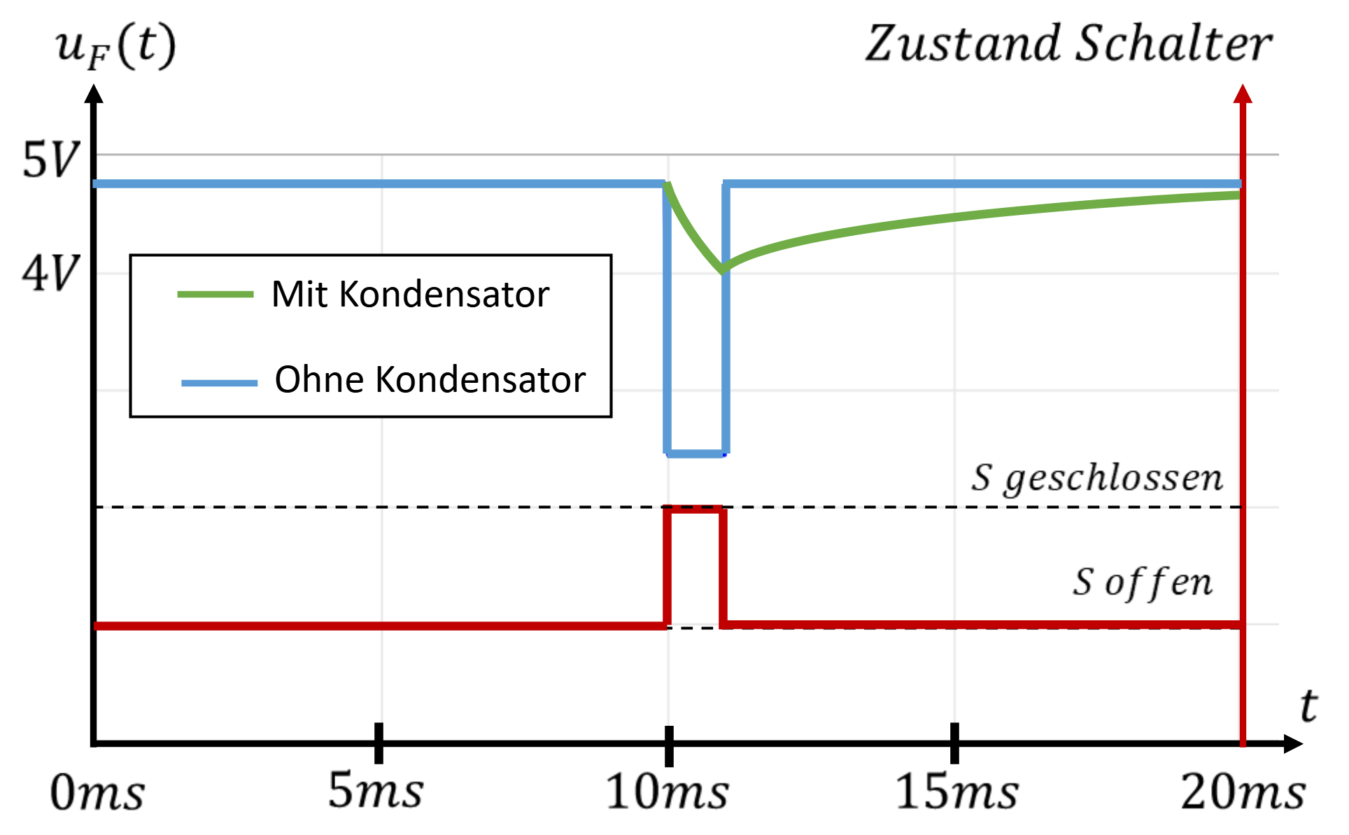
Voltage uF(t) with and without capacitor when switch S is closed briefly — Mit Kondensator = with capacitor · Ohne Kondensator = without capacitor · Zustand = state · Schalter = switch · geschlossen = closed · offen = open

As long as switch S is open, the voltage across the load is 4.76 V, i.e. just under 5 V. When the switch is closed, the voltage across the load without a capacitor jumps to half the voltage, i.e. to 2.38 V (approx. 2.5 V). If a capacitor is used, the voltage only drops to about 4 V. In return, the capacitor must then be recharged. At the far right of the figure, you can see that 10 ms is not quite enough time for this.

The capacitor is discharged and charged via a resistor in each case. It is discharged via R_F and charged via R_i. In both cases, the voltage changes in the form of an exponential function.

\[ \begin{gathered} R_i = R_F = 50\,\Omega \\[4pt] C = 100\,\text{µF} \\[4pt] \tau_{\mathrm{Laden}} = R_i \cdot C = 5\,\mathrm{ms} \\[4pt] \tau_{\mathrm{Entladen}} = R_F \cdot C = 5\,\mathrm{ms} \end{gathered} \]

During recharging (“Laden”), the capacitor voltage reaches 63 % of its final value after τ = 5 ms. Since the capacitor is charged from 4 V to 5 V, the voltage 5 ms after the switch opens is

\[ \begin{gathered} \text{Time the switch opens: } t = 11\,\mathrm{ms} \\[4pt] \tau_{\mathrm{Laden}} = R_i \cdot C = 5\,\mathrm{ms} \\[4pt] \tau_{\mathrm{Laden}} \text{ later: } t = 11\,\mathrm{ms} + 5\,\mathrm{ms} = 16\,\mathrm{ms} \\[4pt] u_C(16\,\mathrm{ms}) = u_C(11\,\mathrm{ms}) + 63\,\% \cdot \Delta U = 4\,\mathrm{V} + 0.63 \cdot 1\,\mathrm{V} = 4.63\,\mathrm{V} \end{gathered} \]

After the time 5 ∙ τ = 25 ms, the capacitor is recharged to 99 % of its maximum value. After that, a new discharge process can start. Since the radio module only transmits once every second, it is ensured that the capacitor is fully charged each time.

Let us look at the discharge process (“Entladen”). The capacitor is discharged by the radio module from 4.76 V towards 2.38 V. Why is that? Once the charging or discharging process is complete, no more current flows at the capacitor. If no current flows out of the capacitor, it has no effect in the circuit. We obtain the voltage and current in a circuit after a completely finished charging or discharging process by mentally removing the capacitor from the circuit. So at the end of the discharge process, the voltage across the load falls to the value to which the light-blue voltage curve falls.

This takes about the time t = 5 ∙ τ = 25 ms. After that, it would be 99 % of the way discharged. However, the discharge process is already stopped after 1 ms, which is why the voltage does not fall all the way to 2.38 V.

To understand the discharge process better, we do not stop it after 1 ms. At the time t = 15 ms in the figure below, the capacitor voltage has fallen by 63 %.

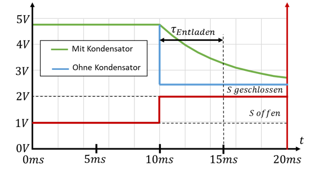
\[ \begin{gathered} \text{Discharge process:} \\[4pt] u_C(10\,\mathrm{ms}) = 4.76\,\mathrm{V} \\[4pt] \tau_{\mathrm{Entladen}} = R_F \cdot C = 5\,\mathrm{ms} \\[4pt] \text{Discharge process: } \Delta U = 4.76\,\mathrm{V} - 2.38\,\mathrm{V} = 2.38\,\mathrm{V} \\[4pt] u_C(15\,\mathrm{ms}) = u_C(10\,\mathrm{ms}) - 0.63 \cdot \Delta U = 4.76\,\mathrm{V} - 1.5\,\mathrm{V} = 3.26\,\mathrm{V} \end{gathered} \]

Voltage uF(t) during discharging with and without capacitor — Entladen = discharging · Mit Kondensator = with capacitor · Ohne Kondensator = without capacitor · geschlossen = closed · offen = open

The challenge is to recognise from which initial value the voltage changes to which final value. The 63 % always refer to the voltage difference ΔU between the initial and final value. It is easy to get confused with the signs here. This is not critical, because you know whether the voltage rises or falls. You can correct the signs of the calculation at the end (also in the exam) if you set them up incorrectly in the formulas.

The discharge process from the second graph does not occur in practice, because discharging is always stopped after 1 ms. By then, the temperature value has already been sent to the smartphone. The second graph only serves to illustrate the discharge process.

When calculating the capacitor size, we assumed that the discharge current is constant during the discharge process. It is not, because the voltage across the load resistor drops over time (green curve). With this incorrect assumption, we dimensioned the capacitance as C = 100 µF. The curves above were simulated with this capacitance. The simulation solves the differential equations and delivers the mathematically exact result. So our approximation was evidently OK, because the voltage across the loads remains above 4 V when the switch is closed for 1 ms.