Complex Power

Circuits with ohmic loads and energy stores generally require active power and reactive power. The active power converts the electrical energy at the ohmic loads into other forms of energy. The reactive power shifts electrical energy back and forth between stores such as inductors and capacitors. The apparent power is the complex sum of both types of power.

The time curves from the last chapter help in understanding the two types of power. For the calculation, we switch back to complex numbers. Active power is purely real. Reactive power is purely imaginary. That is why the complex apparent power is defined as follows:

\[ \begin{gathered} \text{Apparent power } s;\; \text{reactive power } q;\; \text{active power } p \\[4pt] s(\omega) = u(\omega) \cdot i(\omega)^* \\[4pt] s = p + jq \\[4pt] |s| = \sqrt{p^2 + q^2} \\[4pt] p = |s| \cdot \cos(\varphi) \\[4pt] q = |s| \cdot \sin(\varphi) \\[4pt] \varphi = \arctan\left(\frac{q}{p}\right) \\[4pt] \varphi = \varphi_u - \varphi_i \end{gathered} \]

Active and reactive power are calculated from the apparent power via the phase angle φ. It is calculated from the difference between the voltage phase and the current phase.

In complex AC analysis, the apparent power s is calculated as s(ω) = u(ω) ∙ i(ω)^*. The asterisk stands for the mathematical operator “complex conjugate”. For a complex conjugate number, the sign of the imaginary part is reversed. For example, (1+j)^* = 1−j. The active power p(ω) is then defined as the real part of the apparent power and the reactive power q(ω) as its imaginary part. So s = p + jq.

Unfortunately, different units are defined for the three types of power. The apparent power s is given in the unit [s] = V ∙ A. The reactive power q has the unit [q] = var, and the active power has the familiar unit [p] = W.

Physical quantity	Symbol	Unit name	Unit symbol
Apparent power	\(s\)	Volt-ampere	\(\mathrm{VA}\)
Active power	\(p\)	Watt	\(\mathrm{W}\)
Reactive power	\(q\)	Volt-ampere reactive	\(\mathrm{var}\)

As an example, we consider a voltage u(ω) = j3 V and a current i(ω) = 2 A – j2 A.

\[ \begin{gathered} \text{Given: } u(\omega) = j3\,\mathrm{V};\; i(\omega) = 2\,\mathrm{A} - j2\,\mathrm{A} \\[4pt] s(\omega) = u(\omega) \cdot i(\omega)^* = j3\,\mathrm{V} \cdot (2\,\mathrm{A} \textcolor{#c00000}{+} j2\,\mathrm{A}) = j6\,\mathrm{VA} - 6\,\mathrm{VA} \\[4pt] p(\omega) = -6\,\mathrm{W} \\[4pt] q(\omega) = 6\,\mathrm{var} \end{gathered} \]

The reactive power q is always given without the j. The j is contained in the equation s = p + jq. That is why p and q are real. The different units serve to make it immediately clear which type of power is present. As long as we give an apparent power s, the unit is always VA. Only when we then give p or q can we use the units W or var.

An ohmic resistor can only have active power. An energy store can only have reactive power. The reactive power of an inductor is always positive, that of a capacitor always negative. You will find this out yourself when solving problems. It is helpful to know this for checking the results.

Power factor

When you operate electrical installations, for example, you generally want to achieve as much active power as possible. Reactive power is generally undesirable, because it does nothing in the installation; it only recharges stores. How can the proportion of active power in the apparent power be determined easily in practice in order to check how “good” your installation is? For this, we use the power factor.

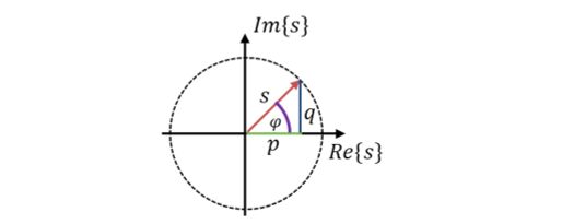
Phasor of the apparent power s in the complex plane with active power p, reactive power q and angle φ

\[ \begin{gathered} \text{Active power: } p = |s| \cdot \cos(\varphi) \\[4pt] \text{100 \% active power: } s = p;\; q = 0;\; \varphi = 0;\; \cos(\varphi) = 1 \\[4pt] \text{Reactive power: } q = |s| \cdot \sin(\varphi) \\[4pt] \text{100 \% reactive power: } s = q;\; p = 0;\; \varphi = \pm\frac{\pi}{2};\; \cos(\varphi) = 0 \end{gathered} \]

In the figure above, the angle φ is drawn between the real axis (x-axis) and the phasor (vector) of the apparent power. In the triangle, it describes how the apparent power is divided into active and reactive power. The proportion of active power p in the apparent power s is expressed by the power factor cos(φ). A “good” installation with little reactive power has a power factor of cos(φ) = 1.

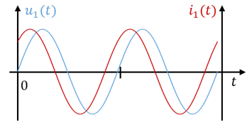
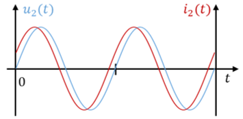
The angle φ of the power equals the phase shift φ between voltage and current. I will show you this with the following example:

\[ \begin{gathered} u(\omega) = 1\,\mathrm{V} \cdot e^{j\frac{\pi}{4}} \text{ with } \varphi_u = \frac{\pi}{4} \\[4pt] i(\omega) = 1\,\mathrm{A} \cdot e^{j\frac{\pi}{2}} \text{ with } \varphi_i = \frac{\pi}{2} \\[4pt] s(\omega) = u(\omega) \cdot i(\omega)^* = 1\,\mathrm{V} \cdot e^{j\frac{\pi}{4}} \cdot 1\,\mathrm{A} \cdot e^{-j\frac{\pi}{2}} = 1\,\mathrm{VA} \cdot e^{\left(j\frac{\pi}{4} - j\frac{\pi}{2}\right)} = 1\,\mathrm{VA} \cdot e^{-j\frac{\pi}{4}} \\[4pt] \varphi = \varphi_u - \varphi_i = \frac{\pi}{4} - \frac{\pi}{2} = -\frac{\pi}{4} \end{gathered} \]

So you can infer the active power by analysing the time curves of voltage and current. You can determine the phase shift between voltage and current from the time difference between the positive zero crossings of the curves. You have to relate this time to the period. The method for determining the phase angle is explained in this chapter.

Then you determine the peak values of voltage and current and multiply them to get the peak value of the apparent power. This peak value multiplied by cos(φ) gives the peak value of the active power.

Two figures of voltage and current curves follow. The peak values of voltage and current are the same in both. That is why the magnitude of the apparent power is also the same in both. The time difference between voltage and current is proportional to their phase shift. The phase angle of the upper curves is larger than that of the lower curves. The proportion of active power in the apparent power is larger in the lower curve than in the upper one.

\[ |s_1| = |s_2| = |s| \]

Voltage u1(t) and current i1(t) with a larger phase shift

\[ \begin{gathered} \varphi_1 = -\frac{\pi}{4} \\[4pt] \cos\left(-\frac{\pi}{4}\right) = 0.71 \\[4pt] p_1 = |s| \cdot 0.71 \end{gathered} \]

Voltage u2(t) and current i2(t) with a small phase shift

\[ \begin{gathered} \varphi_2 = -\frac{\pi}{8} \\[4pt] \cos\left(-\frac{\pi}{8}\right) = 0.92 \\[4pt] p_2 = |s| \cdot 0.92 \\[4pt] p_2 > p_1 \text{ for } |s_1| = |s_2| \end{gathered} \]

Example of a circuit

Let us look at the power delivered by the voltage source in the figure below.

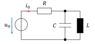
Circuit: source u0 with current i0, resistor R in series with the parallel connection of C and L

\[ \begin{gathered} R = 10\,\Omega \\[4pt] L = 9\,\mathrm{mH} \\[4pt] C = 11\,\mathrm{\mu F} \\[4pt] u_0(\omega) = 10\,\mathrm{V} \\[4pt] \omega = 1\,\mathrm{k}\frac{1}{\mathrm{s}} \end{gathered} \]

First we calculate the current flowing out of the source. For this, the total impedance of the load Z_Ges is formed:

\[ \begin{gathered} Z_{\mathrm{Ges}} = Z_R + (Z_L || Z_C) \\[6pt] (Z_L || Z_C) = \left(\frac{j\omega L \cdot \frac{1}{j\omega C}}{j\omega L + \frac{1}{j\omega C}}\right) = \left(\frac{j\omega L}{j\omega L \cdot j\omega C + 1}\right) = j\left(\frac{\omega L}{1 - \omega^2 LC}\right) \\[6pt] = j\left(\frac{1\,\mathrm{k}\frac{1}{\mathrm{s}} \cdot 9\,\mathrm{mH}}{1 - \left(1\,\mathrm{k}\frac{1}{\mathrm{s}}\right)^2 \cdot 9\,\mathrm{mH} \cdot 11\,\mathrm{\mu F}}\right) = j\left(\frac{9}{1 - 0.1}\right)\Omega = j10\,\Omega \\[6pt] Z_{\mathrm{Ges}} = Z_R + (Z_L || Z_C) = 10\,\Omega + j10\,\Omega = \sqrt{2} \cdot 10\,\Omega \cdot e^{j\frac{\pi}{4}} \\[6pt] i_0(\omega) = \frac{u_0(\omega)}{Z_{\mathrm{Ges}}} = \frac{10\,\mathrm{V}}{\sqrt{2} \cdot 10\,\Omega \cdot e^{j\frac{\pi}{4}}} = \frac{1}{\sqrt{2}}\,\mathrm{A} \cdot e^{-j\frac{\pi}{4}} = \frac{1}{2}\,\mathrm{A}(1 - j) \\[6pt] s(\omega) = u(\omega) \cdot i(\omega)^* = 10\,\mathrm{V} \cdot \frac{1}{\sqrt{2}}\,\mathrm{A} \cdot e^{\textcolor{#c00000}{+}j\frac{\pi}{4}} = \frac{10}{\sqrt{2}}\,\mathrm{VA} \cdot e^{j\frac{\pi}{4}} \\[6pt] \text{Alternatively in component form: } s(\omega) = 10\,\mathrm{V} \cdot \frac{1}{2}\,\mathrm{A}(1 \textcolor{#c00000}{+} j) = 5\,\mathrm{VA}(1 + j) \end{gathered} \]

Simulation

Let us look at the phase angles:

\[ \begin{gathered} \varphi_u = 0 \\[4pt] \varphi_i = -\frac{\pi}{4} \\[4pt] \varphi = \varphi_u - \varphi_i = 0 - \left(-\frac{\pi}{4}\right) = \frac{\pi}{4} \\[4pt] \cos\left(\frac{\pi}{4}\right) = \frac{1}{\sqrt{2}} \end{gathered} \]

This is also the phase angle of the apparent power. The active power equals the power at the resistor, because only reactive power occurs at the inductor and the capacitor. The following applies:

\[ \begin{gathered} p = \mathrm{Re}\{s\} = 5\,\mathrm{W} \\[4pt] \text{Alternatively: } p = |s| \cdot \cos(\varphi) = \frac{10}{\sqrt{2}}\,\mathrm{VA} \cdot \frac{1}{\sqrt{2}} = 5\,\mathrm{W} \end{gathered} \]

Effective power

In electrical engineering, complex quantities always represent peak values and phase. However, the peak value is not a good measure of power, see the chapter Mean value and RMS value. Nobody in practice is interested in the active power as a peak value. If we want to know how hot a hair dryer gets, we always need the effective (RMS) active power. We obtain the effective complex apparent power by substituting voltage and current as RMS values in each case. For sinusoidal voltages and currents, the following applies:

\[ \begin{gathered} u_{\mathrm{eff}} = \frac{\hat{u}}{\sqrt{2}} = \frac{|u|}{\sqrt{2}} \\[6pt] i_{\mathrm{eff}} = \frac{\hat{\imath}}{\sqrt{2}} = \frac{|i|}{\sqrt{2}} \\[6pt] |s_{\mathrm{eff}}| = u_{\mathrm{eff}} \cdot i_{\mathrm{eff}} = \frac{|u|}{\sqrt{2}} \cdot \frac{|i|}{\sqrt{2}} = \frac{|u| \cdot |i|}{2} \end{gathered} \]

The RMS value is a real number, not a complex number. It contains no angle, so it is not a vector. It therefore has no real or imaginary part either. That is why we cannot take the complex conjugate of the RMS current. Once we have determined the apparent power as a peak value, we can easily calculate the effective apparent power with the following formula:

\[ s_{\mathrm{eff}} = \frac{s}{2} \]

The effective apparent power is half as large as the peak value of the apparent power. This is because the peak values of voltage and current have each been divided by √2.

Calculating with apparent power in networks

Suppose you have determined the apparent power of all components in a circuit from their voltage and current values. How can you determine the total apparent power of the circuit? There are two ways of doing this.

You can calculate the apparent power of the source. To do this, you use the voltage and current at the source and calculate exactly as for passive components.

Alternatively, you can add apparent powers. Let us first look at a series connection of two components. As an example, I use resistors in the graphics, but the relationships apply to all types of components. The current through both components is the same. The voltages are added to give a total voltage. The total apparent power of the two components thus results from adding the individual apparent powers. The following applies:

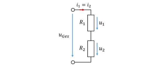
Series connection of R1 and R2 with the same current i1 = i2, partial voltages u1 and u2 and total voltage uGes

\[ \begin{gathered} u_{\mathrm{Ges}}(\omega) = u_1(\omega) + u_2(\omega) \\[4pt] i_1(\omega) = i_2(\omega) = i_{\mathrm{Ges}}(\omega) \\[4pt] s_1(\omega) = u_1 \cdot i_{\mathrm{Ges}}^*(\omega) \\[4pt] s_2(\omega) = u_2 \cdot i_{\mathrm{Ges}}^*(\omega) \\[4pt] s_{\mathrm{Ges}}(\omega) = u_{\mathrm{Ges}} \cdot i_{\mathrm{Ges}}^*(\omega) = u_1 \cdot i_{\mathrm{Ges}}^*(\omega) + u_2 \cdot i_{\mathrm{Ges}}^*(\omega) = s_1(\omega) + s_2(\omega) \end{gathered} \]

In a series connection, the apparent powers of the components add up to that of the whole circuit.

Next, let us look at a parallel connection:

Parallel connection of R1 and R2 with the same voltage, partial currents i1 and i2 and total current iGes — Ges = total

\[ \begin{gathered} u_{\mathrm{Ges}}(\omega) = u_1(\omega) = u_2(\omega) \\[4pt] i_{\mathrm{Ges}}(\omega) = i_1(\omega) + i_2(\omega) \\[4pt] s_1(\omega) = u_{\mathrm{Ges}} \cdot i_1^*(\omega) \\[4pt] s_2(\omega) = u_{\mathrm{Ges}} \cdot i_2^*(\omega) \\[4pt] s_{\mathrm{Ges}}(\omega) = u_{\mathrm{Ges}} \cdot i_{\mathrm{Ges}}^*(\omega) = u_{\mathrm{Ges}} \cdot i_1^*(\omega) + u_{\mathrm{Ges}} \cdot i_2^*(\omega) = s_1(\omega) + s_2(\omega) \end{gathered} \]

The total apparent power of two components connected in parallel also equals the sum of the apparent powers of the components.

In a series connection, the current is the same in both components and the voltages of both components are added. In a parallel connection, the voltage is the same across both components and the currents of both components are added. Both lead to the apparent powers of the components being added to give the total apparent power.

Evidently, it does not matter how components are connected. You can always add the apparent powers of all components and obtain the total apparent power of the circuit.

Summary

If we measure voltage and current in the time domain and multiply them, we obtain the instantaneous power u(t) ∙ i(t). Its time average equals the effective active power. The component with zero mean that oscillates at twice the frequency contains the reactive power. In the time domain, these quantities are difficult to separate.

We look at the complex quantities u(ω) and i(ω)*. If we multiply them, we obtain the complex apparent power s(ω). The real part of the apparent power equals the active power p(ω), the imaginary part the reactive power q(ω). If the apparent power is available as a complex number in component form, you can therefore easily read off the active and reactive components from s(ω) = p(ω) + jq(ω).

We obtain the proportion of active power in the apparent power from cos(φ) = p(ω) / |s(ω)|. The angle φ equals the phase shift between voltage and current.