Measurement Technology › Differential Signals

Half-Bridge

Differential signals are often used to remove an offset from a signal. I will show you this using the example of the PT100, which has this ugly offset of 100 Ω. The PT100 is used in the following bridge circuit:

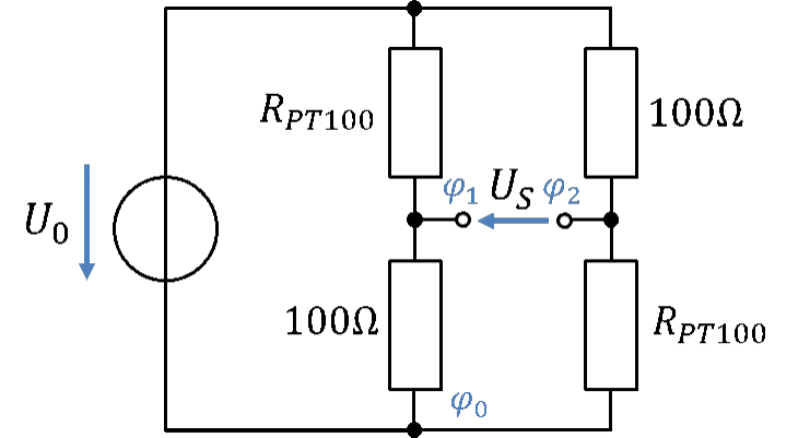
Bridge circuit of two voltage dividers, each with a PT100 and 100 Ω, bridge voltage U_S between the potentials φ1 and φ2

The circuit is supplied by a voltage source U₀. It consists of two voltage dividers, each with a resistor R = 100 Ω and a PT100. The potentials in the middle of the voltage dividers, φ₂ and φ₁, correspond to the weights on the balance.

I call the output voltage of the bridge circuit the sensor voltage U_S, because it is the input voltage of the analogue signal processing. It lies between the potentials φ₂ and φ₁. Neither of the two potentials is at ground.

Explanation of the function

First, let us look at the two voltage dividers. For the calculation we use the formulas from the fundamentals of electrical engineering.

\[ \begin{gathered} \text{General:} \\[6pt] R_{\mathrm{PT100}} = 100\,\Omega + 0.4\,\frac{\Omega}{°\mathrm{C}} \cdot T \\[6pt] \text{Left voltage divider: } \varphi_1 = U_0 \cdot \frac{100\,\Omega}{100\,\Omega + R_{\mathrm{PT100}}} \\[6pt] \text{Right voltage divider: } \varphi_2 = U_0 \cdot \frac{R_{\mathrm{PT100}}}{100\,\Omega + R_{\mathrm{PT100}}} \end{gathered} \]

Next, let us look at the circuit at the temperature T = 0 °C. Then the following applies:

\[ \begin{gathered} T = 0\,°\mathrm{C}\text{:} \\[6pt] R_{\mathrm{PT100}} = 100\,\Omega + 0.4\,\frac{\Omega}{°\mathrm{C}} \cdot 0\,°\mathrm{C} = 100\,\Omega \\[6pt] \text{Left voltage divider: } \varphi_1 = U_0 \cdot \frac{100\,\Omega}{100\,\Omega + 100\,\Omega} = \frac{U_0}{2} \\[6pt] \text{Right voltage divider: } \varphi_2 = U_0 \cdot \frac{R_{\mathrm{PT100}}}{100\,\Omega + R_{\mathrm{PT100}}} = \frac{U_0}{2} \\[6pt] U_S = \varphi_2 - \varphi_1 = \frac{U_0}{2} - \frac{U_0}{2} = 0\,\mathrm{V} \\[6pt] \text{The balance is level: } \varphi_1 = \varphi_2 \end{gathered} \]

At T = 0 °C, the sensor voltage is 0 V. The balance is level; both weights are equal. φ₂ = φ₁ applies. The resistor R = 100 Ω was chosen precisely so that the balance is level at T = 0 °C. We say that the bridge is “balanced” at T = 0 °C. A bridge is balanced when its output voltage is 0 V.

What happens when the temperature changes? How does this affect the potentials? Let us look at the voltage dividers again:

\[ \begin{gathered} \text{General:} \\[6pt] R_{\mathrm{PT100}} = 100\,\Omega + 0.4\,\frac{\Omega}{°\mathrm{C}} \cdot T \\[6pt] \text{Left voltage divider:} \\[6pt] \varphi_1 = U_0 \cdot \frac{100\,\Omega}{100\,\Omega + R_{\mathrm{PT100}}} = U_0 \cdot \frac{100\,\Omega}{100\,\Omega + \left(100\,\Omega + 0.4\,\frac{\Omega}{°\mathrm{C}} \cdot T\right)} = U_0 \cdot \frac{100\,\Omega}{200\,\Omega + 0.4\,\frac{\Omega}{°\mathrm{C}} \cdot T} \\[6pt] \text{Right voltage divider:} \\[6pt] \varphi_2 = U_0 \cdot \frac{R_{\mathrm{PT100}}}{100\,\Omega + R_{\mathrm{PT100}}} = U_0 \cdot \frac{100\,\Omega + 0.4\,\frac{\Omega}{°\mathrm{C}} \cdot T}{100\,\Omega + \left(100\,\Omega + 0.4\,\frac{\Omega}{°\mathrm{C}} \cdot T\right)} = U_0 \cdot \frac{100\,\Omega + 0.4\,\frac{\Omega}{°\mathrm{C}} \cdot T}{200\,\Omega + 0.4\,\frac{\Omega}{°\mathrm{C}} \cdot T} \end{gathered} \]

As the temperature T rises, the denominator of φ₁ becomes larger. So φ₁ becomes smaller. For φ₂, the analysis is more difficult. Overall, the fraction becomes larger. I prefer to show this with a numerical example rather than in general:

\[ \begin{gathered} \text{For the example: set } U_0 = 10\,\mathrm{V} \\[6pt] T = 100\,°\mathrm{C} \rightarrow R_{\mathrm{PT100}} = 100\,\Omega + 0.4\,\frac{\Omega}{°\mathrm{C}} \cdot 100\,°\mathrm{C} = 140\,\Omega \\[6pt] \text{Left voltage divider: } \varphi_1 = 10\,\mathrm{V} \cdot \frac{100\,\Omega}{100\,\Omega + 140\,\Omega} = 4.17\,\mathrm{V} \\[6pt] \text{Right voltage divider: } \varphi_2 = 10\,\mathrm{V} \cdot \frac{140\,\Omega}{100\,\Omega + 140\,\Omega} = 5.83\,\mathrm{V} \\[6pt] U_S = \varphi_2 - \varphi_1 = 5.83\,\mathrm{V} - 4.17\,\mathrm{V} = 1.67\,\mathrm{V} \end{gathered} \]

Simulation

\[ \begin{gathered} T = -100\,°\mathrm{C} \rightarrow R_{\mathrm{PT100}} = 60\,\Omega \\[6pt] \text{Left voltage divider: } \varphi_1 = 10\,\mathrm{V} \cdot \frac{100\,\Omega}{100\,\Omega + 60\,\Omega} = 6.25\,\mathrm{V} \\[6pt] \text{Right voltage divider: } \varphi_2 = 10\,\mathrm{V} \cdot \frac{60\,\Omega}{100\,\Omega + 60\,\Omega} = 3.75\,\mathrm{V} \\[6pt] U_S = \varphi_2 - \varphi_1 = 3.75\,\mathrm{V} - 6.25\,\mathrm{V} = -2.5\,\mathrm{V} \end{gathered} \]

At positive temperatures, the output voltage of the bridge rises. In the right voltage divider, the potential φ₂ rises. In the left voltage divider, the potential φ₁ falls.

At negative temperatures, the output voltage of the bridge falls. In the right voltage divider, the potential φ₂ falls. In the left voltage divider, the potential φ₁ rises.

Calculating the output voltage

The explanation so far is mainly for your understanding. To calculate the output voltage, we use the following formula directly:

\[ \begin{gathered} U_S = \varphi_2 - \varphi_1 = U_0 \cdot \frac{100\,\Omega + 0.4\,\frac{\Omega}{°\mathrm{C}} \cdot T}{200\,\Omega + 0.4\,\frac{\Omega}{°\mathrm{C}} \cdot T} - U_0 \cdot \frac{100\,\Omega}{200\,\Omega + 0.4\,\frac{\Omega}{°\mathrm{C}} \cdot T} = U_0 \cdot \frac{0.4\,\frac{\Omega}{°\mathrm{C}} \cdot T}{200\,\Omega + 0.4\,\frac{\Omega}{°\mathrm{C}} \cdot T} \\[6pt] U_S = U_0 \cdot \frac{0.4\,\frac{\Omega}{°\mathrm{C}} \cdot T}{200\,\Omega + 0.4\,\frac{\Omega}{°\mathrm{C}} \cdot T} \end{gathered} \]

Approximation

Assuming that the value 200 Ω in the denominator is much larger than the change in resistance with temperature, we use the following approximation:

\[ \begin{gathered} U_S = U_0 \cdot \frac{0.4\,\frac{\Omega}{°\mathrm{C}} \cdot T}{200\,\Omega + 0.4\,\frac{\Omega}{°\mathrm{C}} \cdot T} \approx U_0 \cdot \frac{0.4\,\frac{\Omega}{°\mathrm{C}} \cdot T}{200\,\Omega} \\[6pt] \text{With } R = 100\,\Omega \text{ (fixed resistor) and} \\[6pt] \Delta R = 0.4\,\frac{\Omega}{°\mathrm{C}} \cdot T \text{ (variable resistance), the following applies:} \\[6pt] R_{\mathrm{PT100}} = R + \Delta R \\[6pt] U_S \approx U_0 \cdot \frac{\Delta R}{2R} \end{gathered} \]

This simplification only applies if the temperature changes only slightly. For temperature measurement systems with a very large measuring range, the simplification cannot be used.

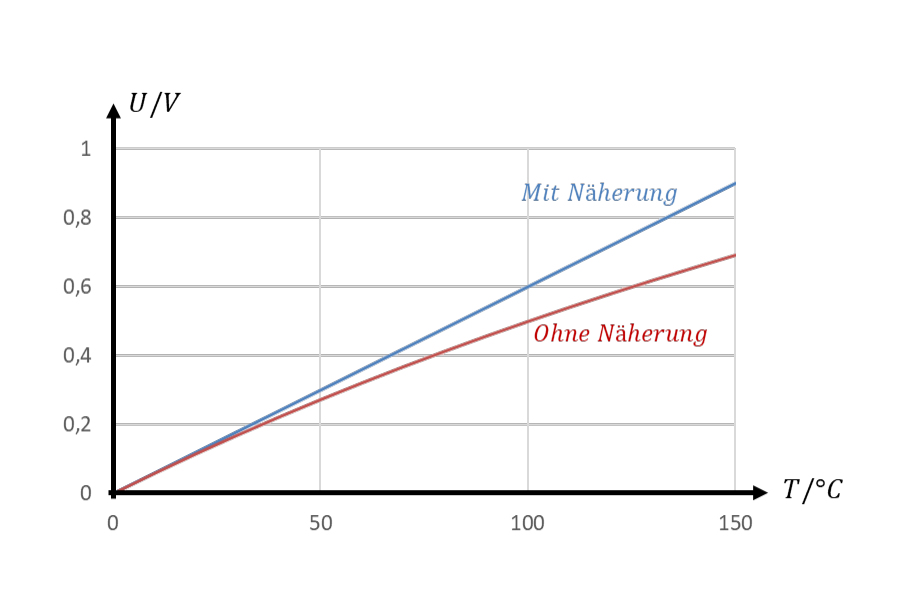
The result is a linear expression of the type y = m ∙ x + b with b = 0. A straight-line equation with b = 0 represents a proportional relationship. That is the only reason why we use this approximation ;-). This expression yields (with and without approximation) the following curve of voltage against temperature:

Bridge voltage against temperature with and without approximation: the approximation is good for small temperatures — Näherung = approximation

The output voltage of the bridge circuit with PT100 has no offset. That is good. The real orange curve is non-linear. The blue curve with approximation is proportional. The deviation of the real orange curve from the approximated blue curve can easily be corrected in digital signal processing. For calculations in this chapter, we only use the approximation from now on. Even without the approximation, this curve comes closer to our goal from the chapter Measuring resistors than the attempts with the voltage divider and the current source.

Transfer function

The transfer function can only be given in the approximated form, because only then is the behaviour proportional. The following applies:

\[ H = \frac{U_S}{T} \approx U_0 \cdot \frac{\frac{0.4\,\frac{\Omega}{°\mathrm{C}} \cdot T}{200\,\Omega}}{T} = U_0 \cdot \frac{0.4\,\frac{\Omega}{°\mathrm{C}}}{200\,\Omega} = U_0 \cdot 2\,\mathrm{m}\,\frac{1}{°\mathrm{C}} \]

The transfer function corresponds to the slope of the characteristic curve. It indicates how strongly the output voltage changes with temperature. The slope depends only on U₀. In practice, we cannot make this value arbitrarily large. That is why we need amplifiers here too, in order to make optimal use of the input voltage range of the ADC.