Measurement Technology › Filters Part 2 › Filter Types

Low-Pass Filter

A low-pass filter is described mathematically as

\[ |H(\omega)| = \frac{1}{\sqrt{1 + (\omega RC)^2}} = \frac{1}{\sqrt{1 + (\omega/\omega_g)^2}} \]

Electrical circuits that behave according to this formula have a low-pass characteristic. In the last chapter you already got to know a passive low-pass filter made of a resistor and a capacitor. A passive filter can only reduce peak values, not increase them. Active filters can amplify and attenuate signals.

The following circuit combines an inverting op-amp amplifier with a low-pass filter. So far we have only considered resistors in op-amp circuits. For filters, however, we need storage elements. That is why we now again consider complex impedances or reactances instead of the resistors. You already know the routine: first the analysis with impedances for ETR, then the analysis with reactances for BMT / UFC. The following applies:

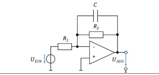
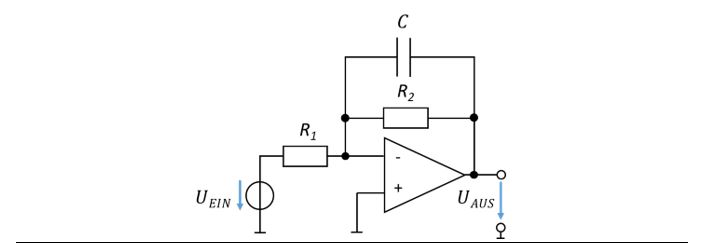
Active low-pass filter: inverting amplifier with capacitor C in parallel with R_2

\[ \begin{gathered} \text{Analysis with impedances:} \\[6pt] \underline{H}(\omega) = -\frac{\underline{Z}_2}{\underline{Z}_1} = -\frac{\underline{Z}_{R2} \parallel \underline{Z}_C}{\underline{Z}_{R1}} \\[6pt] \text{with } \underline{Z}_{R2} = R_2,\ \underline{Z}_{R1} = R_1 \text{ and } \underline{Z}_C = \frac{1}{j\omega C} \text{:} \\[6pt] \underline{Z}_{R2} \parallel \underline{Z}_C = \frac{R_2 \cdot \frac{1}{j\omega C}}{R_2 + \frac{1}{j\omega C}} = \frac{R_2}{1 + j\omega R_2 C} \\[6pt] \underline{H}(\omega) = -\frac{\underline{Z}_2}{\underline{Z}_1} = -\frac{\frac{R_2}{1 + j\omega R_2 C}}{R_1} = -\frac{R_2}{R_1(1 + j\omega R_2 C)} = -\frac{R_2}{R_1} \cdot \left(\frac{1}{1 + j\omega R_2 C}\right) \\[6pt] \underline{H}(\omega) = \underbrace{-\frac{R_2}{R_1}}_{\text{gain } v} \cdot \underbrace{\left(\frac{1}{1 + j\omega R_2 C}\right)}_{\text{filter}} = v \cdot \left(\frac{1}{1 + j\omega/\omega_g}\right) \end{gathered} \]

\[ \begin{gathered} \text{Analysis with reactances:} \\[6pt] |H| = -\frac{X_2}{X_1} = -\frac{R_2 \parallel X_C}{R_1} \\[6pt] \text{with } X_C = \frac{1}{\omega C} \text{:} \\[6pt] R_2 \parallel X_C = \frac{R_2 \cdot \frac{1}{\omega C}}{\sqrt{(R_2)^2 + \left(\frac{1}{\omega C}\right)^2}} = \frac{R_2}{\sqrt{(R_2 \cdot \omega C)^2 + 1}} = \frac{R_2}{\sqrt{1 + (\omega R_2 C)^2}} \\[6pt] H(\omega) = -\frac{X_2}{X_1} = -\frac{\frac{R_2}{\sqrt{(\omega R_2 C)^2 + 1}}}{R_1} = -\frac{R_2}{R_1} \cdot \frac{1}{\sqrt{1 + (\omega R_2 C)^2}} = -\frac{R_2}{R_1} \cdot \frac{1}{\sqrt{1 + (\omega/\omega_g)^2}} \text{ with } \omega_g = \frac{1}{R_2 C} \\[6pt] H(\omega) = \underbrace{-\frac{R_2}{R_1}}_{\text{gain } v} \cdot \underbrace{\frac{1}{\sqrt{1 + (\omega R_2 C)^2}}}_{\text{filter}} = v \cdot \frac{1}{\sqrt{1 + (\omega/\omega_g)^2}} \end{gathered} \]

The transfer function consists of the gain term of the classic inverting amplifier multiplied by the transfer function of a low-pass filter.

The gain v is set by the two resistors. The cut-off frequency is determined by the components between the op-amp output and the inverting input: by R₂ and C. For the circuit above:

\[ \begin{gathered} v = -\frac{R_2}{R_1},\quad \omega_g = \frac{1}{R_2 C} \\[6pt] H(\omega) = v \cdot H_{\mathrm{Filter}}(\omega) \end{gathered} \]

Example

A sensor signal is made up of a useful component (depending on the physical quantity) and an interference component. The following applies (Nutz = useful, Stör = interference):

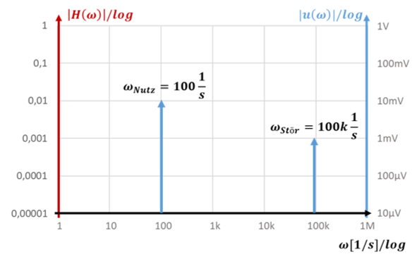
\[ \begin{gathered} u_{\mathrm{Sensor}} = u_{\mathrm{Nutz}} + u_{\mathrm{Stör}} \\[6pt] u_{\mathrm{Nutz}}(t) = 10\,\mathrm{mV} \cdot \sin(\omega_{\mathrm{Nutz}} \cdot t),\quad \omega_{\mathrm{Nutz}} = 100\,\tfrac{1}{\mathrm{s}} \\[6pt] u_{\mathrm{Nutz}} = [-10\,\mathrm{mV} \ldots 10\,\mathrm{mV}] \\[6pt] u_{\mathrm{Stör}}(t) = 1\,\mathrm{mV} \cdot \sin(\omega_{\mathrm{Stör}} \cdot t),\quad \omega_{\mathrm{Stör}} = 100\mathrm{k}\,\tfrac{1}{\mathrm{s}} \\[6pt] \text{Goal: } u_{\mathrm{Aus,OP}} = [-3\,\mathrm{V} \ldots 3\,\mathrm{V}] \end{gathered} \]

Spectrum: useful signal at 100 1/s with 10 mV, interference signal at 100k 1/s with 1 mV — Nutz = useful

In filter problems, we ignore the shifting of signals; we only consider amplification and filtering. This reduces complexity and makes real problems easier to calculate. We reduce even further: only the magnitude of the gain is considered, not the sign and no phase rotation with j.

Task: Draw and dimension a circuit that optimally maps the useful signal to the target voltage range and attenuates the interference as much as possible. Set R₂ = 300 kΩ.

Solution: First we calculate the required gain. With v = +300 or v = −300, the range of the useful voltage is mapped correctly to the range of the output voltage. You can multiply both range limits of the useful signal by the factors and obtain the range limits of the output signal in each case. Two solutions are possible. Since filters in this tutorial are always built with inverting amplifiers, we choose v = −300.

We set the cut-off frequency a factor of 10 higher than the useful frequency, at ω_g = 1k 1/s.

We implement this mathematical function with the following filter circuit:

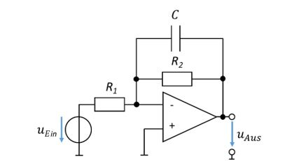
Active low-pass filter with R_1, R_2 and C — Aus = out (output)

\[ \begin{gathered} v = -\frac{R_2}{R_1} = -300;\quad R_1 = \frac{R_2}{300} = \frac{300\,\mathrm{k\Omega}}{300} = 1\,\mathrm{k\Omega} \\[6pt] \omega_g = \frac{1}{R_2 C} = 1\mathrm{k}\,\frac{1}{\mathrm{s}};\quad C = \frac{1}{R_2 \omega_g} = \frac{1}{300\,\mathrm{k\Omega} \cdot 1\mathrm{k}\,\frac{1}{\mathrm{s}}} = 3.33\,\mathrm{nF} \\[6pt] |H| = -\frac{R_2}{R_1} \cdot \frac{1}{\sqrt{1 + \left(\frac{\omega}{\omega_g}\right)^2}} = v \cdot |H_{\mathrm{Filter}}| \end{gathered} \]

Simulation

You calculate the gain from the ratio of the resistors. You calculate the cut-off frequency from the components across the op-amp.

The gain or attenuation of the two signals can be calculated from the transfer function. Alternatively – much more simply – it can be read from the Bode plot.

Calculating the transfer function

The transfer function is made up of filtering and gain.

\[ \begin{gathered} |H(\omega)| = \left|v \cdot \frac{1}{\sqrt{1 + (\omega/\omega_g)^2}}\right| = \left|-300 \cdot \left(\frac{1}{\sqrt{1 + \left(\omega/(1\mathrm{k}\,\frac{1}{\mathrm{s}})\right)^2}}\right)\right| \\[6pt] |H(\omega_{\mathrm{Nutz}})| = \left|-300 \cdot \left(\frac{1}{\sqrt{1 + \left(\frac{100\,1/\mathrm{s}}{1\mathrm{k}\,1/\mathrm{s}}\right)^2}}\right)\right| = \left|-300 \cdot \left(\frac{1}{\sqrt{1 + (0.1)^2}}\right)\right| \approx |-300 \cdot 1| = 300 \\[6pt] |H(\omega_{\mathrm{Stör}})| = \left|-300 \cdot \left(\frac{1}{\sqrt{1 + \left(\frac{100\mathrm{k}\,1/\mathrm{s}}{1\mathrm{k}\,1/\mathrm{s}}\right)^2}}\right)\right| = \left|-300 \cdot \left(\frac{1}{\sqrt{1 + (100)^2}}\right)\right| \approx \left|-300 \cdot \frac{1}{100}\right| = 3 \end{gathered} \]

The calculation is possible but mathematically laborious. You can read off the gain much more easily in the Bode plot. In the exam you do not need to calculate; reading off is always sufficient. Nobody does this calculation voluntarily…

Reading the gain from the Bode plot

v = −300 applies to all signals. Depending on its frequency, each signal is additionally multiplied by a filter factor. We stay with the numerical example from above. The following figure shows the Bode plot in which gain and filtering are combined:

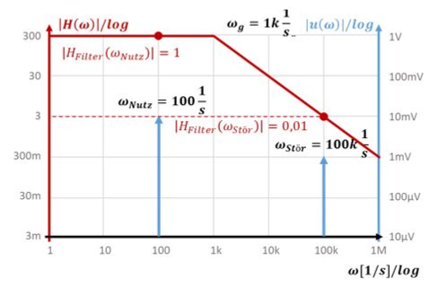
Bode plot of the active low-pass filter: gain 300 in the pass band, 3 at the interference signal — Nutz = useful

\[ \begin{gathered} |H(\omega_{\mathrm{Nutz}})| = 300 \\[6pt] |H(\omega_{\mathrm{Stör}})| = 3 \end{gathered} \]

Once you have drawn the Bode plot, you can read off the values very easily. The art therefore lies in drawing the Bode plot of a filter. To do this, you use the base gain in the pass band and reduce this gain value in the attenuation range. The base gain in the pass band is 1 for passive filters without an op-amp and −R₂/R₁ for filters with an op-amp. Since we consider magnitudes, the minus sign is dropped.

Signal-to-noise ratio

An important measure for assessing a filter is the signal-to-noise ratio (SNR). It describes how strongly a useful signal is affected by interference. Mathematically, it indicates by what factor the peak value of the useful signal is larger than the peak value of the interference signal. A large signal-to-noise ratio is therefore good. We obtain the signal-to-noise ratio from the magnitude of the ratio of the peak values. Let us look again at the example from above:

\[ \begin{gathered} u_{\mathrm{Nutz}}(t) = 10\,\mathrm{mV} \cdot \sin(\omega t) \rightarrow u_{\mathrm{Nutz}}(\omega) = 10\,\mathrm{mV} \\[6pt] u_{\mathrm{Stör}}(t) = 1\,\mathrm{mV} \cdot \sin(\omega t) \rightarrow u_{\mathrm{Stör}}(\omega) = 1\,\mathrm{mV} \\[6pt] u_{\mathrm{Sensor}}(\omega) = u_{\mathrm{Nutz}}(\omega) + u_{\mathrm{Stör}}(\omega) \end{gathered} \]

At the output of the op-amp:

\[ \begin{gathered} u_{\mathrm{Aus,OP}}(\omega) = H(\omega) \cdot u_{\mathrm{Sensor}}(\omega) \\[6pt] H(\omega) = v \cdot H_{\mathrm{Filter}}(\omega) \\[6pt] H(\omega_{\mathrm{Nutz}}) = 300 \\[6pt] H(\omega_{\mathrm{Stör}}) = 3 \\[6pt] u_{\mathrm{Aus,OP,Nutz}}(\omega) = H(\omega_{\mathrm{Nutz}}) \cdot u_{\mathrm{Nutz}}(\omega) = 300 \cdot 10\,\mathrm{mV} = 3\,\mathrm{V} \\[6pt] u_{\mathrm{Aus,OP,Stör}}(\omega) = H(\omega_{\mathrm{Stör}}) \cdot u_{\mathrm{Stör}}(\omega) = 3 \cdot 1\,\mathrm{mV} = 3\,\mathrm{mV} \end{gathered} \]

The complex form of the signal as a function of ω gives the peak value directly. 1 mV of interference peak value becomes 3 mV at the output of the op-amp. 10 mV of useful signal peak value becomes 3 V. The useful signal is amplified much more than the interference signal. We can calculate the signal-to-noise ratio (SSA in the formulas, from German “Signal-Störabstand”) in the sensor voltage and at the output of the op-amp to determine how well the circuit does its job:

\[ \begin{gathered} \mathrm{SSA}_{\mathrm{Sensor}} = \frac{|\hat{u}_{\mathrm{Nutz}}(\omega_{\mathrm{Nutz}})|}{|\hat{u}_{\mathrm{Stör}}(\omega_{\mathrm{Stör}})|} = \frac{10\,\mathrm{mV}}{1\,\mathrm{mV}} = 10 \\[6pt] \mathrm{SSA}_{\mathrm{Ausgang\ OP}} = \frac{|\hat{u}_{\mathrm{Aus,OP,Nutz}}(\omega)|}{|\hat{u}_{\mathrm{Aus,OP,Stör}}(\omega)|} = \frac{3\,\mathrm{V}}{3\,\mathrm{mV}} = 1000 \end{gathered} \]

The circuit increases the “distance” between useful and interference signal by a factor of 100. If we look at such a good “interference suppression” by a factor of 100 in a time plot, it looks like this:

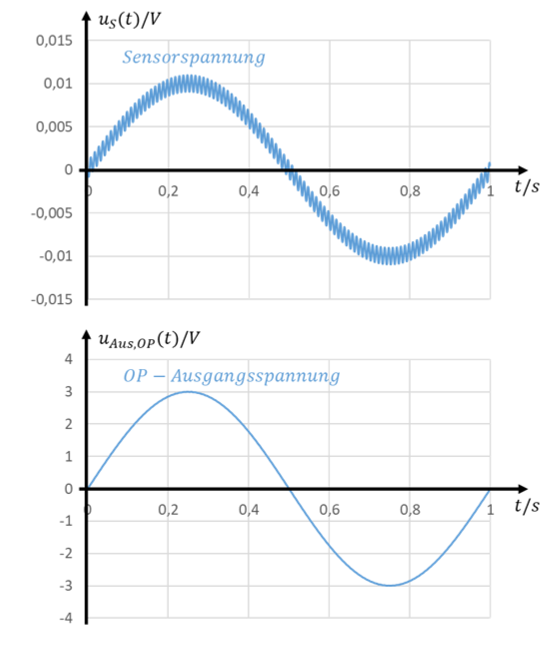
Sensor voltage with superimposed interference and filtered, amplified op-amp output voltage between −3 V and 3 V — Sensorspannung = sensor voltage · Ausgangsspannung = output voltage

Low-pass filters can also be built with inductors as storage elements. In op-amp circuits in measurement technology, capacitors are preferred because they do not disturb the rest of the circuit with stray fields and are considerably cheaper and smaller than inductors.

Passive low-pass filters are built only from passive components – i.e. inductors, capacitors and resistors. These filters can only attenuate the amplitude of signals or let them pass. If a signal is to be amplified at the same time, active filters with op-amp circuits must be used. If a signal has to be amplified anyway, it is very easy to filter it as well. You only need to add a capacitor.

Note: the cut-off frequency and the gain do not depend on the circuit structure. You set these parameters with the components. That is why the gain and cut-off frequency in both circuits are only example values.

Note: Determining the signal-to-noise ratio is often an exam task that gives a particularly large number of points.