Disturbances After the Integrator

If a disturbance acts to the right of the plant’s integrator, you are in luck, because then the integrator already rejects the disturbance. In the steady state, the disturbance then has no effect at all on the controlled variable. To illustrate this, we consider an I system with a P controller with K_PR = 1. A disturbance d acts directly on the controlled variable.

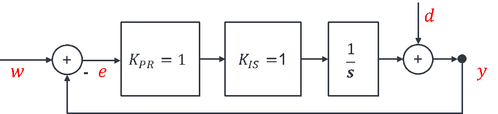
Control loop with K_PR = 1, K_IS = 1 and integrator 1/s, disturbance d acts behind the integrator at the output

\[ \begin{gathered} y = d + K_{PR} \cdot K_{IS} \cdot \frac{1}{s} \cdot e \\[6pt] e = w - y = -y \text{ with } w = 0 \\[6pt] y = d + K_{PR} \cdot K_{IS} \cdot \frac{1}{s} \cdot (-y) \\[6pt] y \left(1 + K_{PR} \cdot K_{IS} \cdot \frac{1}{s}\right) = d \\[6pt] y = \frac{d}{1 + K_{PR} \cdot K_{IS} \cdot \frac{1}{s}} \xrightarrow[s = 0]{} \frac{d}{1 + \infty} = 0 \\[6pt] H_{\mathrm{SU}} = \frac{y}{d} = 0 \end{gathered} \]

The plant’s integrator already ensures that the disturbance rejection is ideal, so the disturbance has no effect at all on the controlled variable. No further integrator is needed in the controller to ensure e = 0.

\[ \begin{gathered} H_{\mathrm{Links}} = A \text{ (in this special case)} \\[6pt] H_{\mathrm{Links}} = A = K_{PR} \cdot K_{IS} \cdot \frac{1}{s} \\[6pt] y \approx \frac{1}{H_{\mathrm{Links}}} \cdot d \\[6pt] H_{\mathrm{SU}} = \frac{y}{d} \approx \frac{1}{H_{\mathrm{Links}}} = \frac{s}{K_{PR} \cdot K_{IS}} \end{gathered} \]

The general solution, in which the disturbance does not have to be to the right of the integrator, is explained in one of the previous chapters. Let us look at a numerical example for this case. I have added two signals g and u.

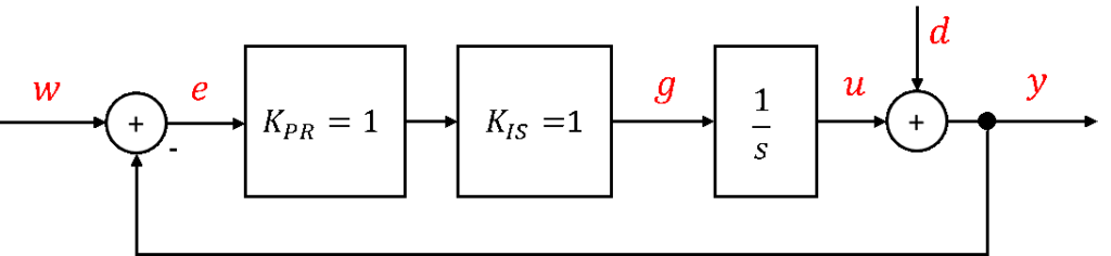
Control loop with intermediate variables g before and u after the integrator, disturbance d at the output

We start with a steady state with example values. For y = w, u = w – d must hold. Then y = u + d becomes y = (w – d) + d = w. How large must g be so that u = w – d? Since u is the output of an integrator, the input g must be 0 in the steady state. If the input g were ≠ 0, the output would keep changing and the state would not (yet) be steady.

The output of an integrator can take almost any value in the steady state. There are only two restrictions: the limited fill level of the storage element in practice and the sign of the output. If the input is always positive, the output can only be positive as well. Let us insert numbers:

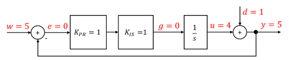
\[ \begin{gathered} w = 5 \text{ and } d = 1 \\[6pt] \text{Steady state: } g = 0 \\[6pt] g = K_{PR} \cdot K_{IS} \cdot e \rightarrow g = e = 0 \\[6pt] e = w - y \text{ with } e = 0 \rightarrow y = w \rightarrow y = 5 \\[6pt] y = d + u \rightarrow u = y - d = 5 - 1 \rightarrow u = 4 \end{gathered} \]

Control loop in the steady state with w = 5, d = 1: e = 0, g = 0, u = 4, y = 5

The control loop remains in the steady state with unchanged values. The control error e is 0 and the output y is non-zero. This is only possible when storage elements are used.

Now the disturbance d changes stepwise from 1 to 2. The state of the system changes, so it is no longer steady. What happens?

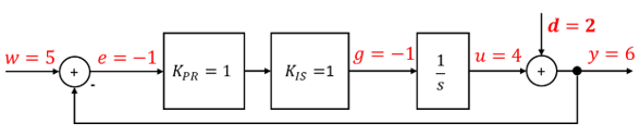
\[ \begin{gathered} w = 5 \text{ and } d = 2 \\[6pt] u = 4 \text{ from the old solution} \rightarrow y = u + d = 6 \\[6pt] e = w - y = 5 - 6 = -1 \\[6pt] g = K_{PR} \cdot K_{IS} \cdot e \rightarrow g = e = -1 \end{gathered} \]

Control loop directly after the disturbance step to d = 2: u = 4, y = 6, e = g = −1

The value g = -1 is applied to the input of the storage element. The output value u of the storage element therefore decreases continuously until the system has settled to new constant values. During the transition between the two states, u changes continuously. Let us look at an arbitrary intermediate step at which u has just reached the value 3.5:

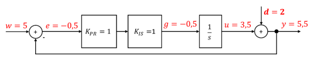
\[ \begin{gathered} u = u_0 + \int g(t)\,dt = 4 + \int (-1)\,dt = 3.5 \\[6pt] y = u + d = 3.5 + 2 = 5.5 \\[6pt] e = w - y = 5 - 5.5 = -0.5 \\[6pt] g = e = -0.5 \end{gathered} \]

Control loop in the next step: u = 3.5, y = 5.5, e = g = −0.5

The storage element is now driven at its input with only g = -0.5. The output of the storage element decreases more slowly than at the beginning. Finally, in the steady state:

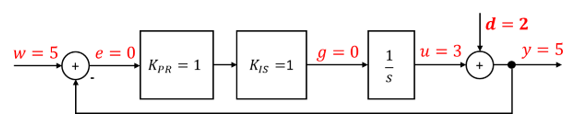
\[ \begin{gathered} u = u_0 + \int g(t)\,dt = 3.5 + \int (-0.5)\,dt = 3 \\[6pt] y = u + d = 3 + 2 = 5 \\[6pt] e = w - y = 5 - 5 = 0 \\[6pt] g = e = 0 \end{gathered} \]

Control loop in the new steady state: u = 3, y = 5, e = g = 0

The storage element is driven negatively at its input until its output u has reached the “right” value u = 3. The drive g at the storage input becomes less and less negative over time, so the output u decreases more and more slowly. This results in PT-1 behaviour.

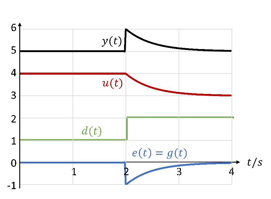
Time curves of y(t), u(t), d(t) and e(t) = g(t) for the disturbance step from d = 1 to d = 2 at t = 2 s

The figure above shows the time curves of y(t), u(t), d(t) and e(t) when d(t) steps from 1 to 2 at time t = 2 s. This is immediately followed by a step in the control error e(t), which then decays. This signal is applied to the input of the integrator as g(t) = e(t). The output of the integrator u(t) decreases as long as g(t) at its input is negative. The controlled variable y is briefly too high until u(t) has dropped from 4 to 3.